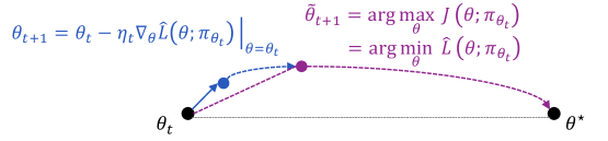
## Diagram: Gradient-Based Optimization Process ### Overview The image depicts a mathematical optimization process involving parameter updates and trajectory visualization. It combines equations describing iterative updates with a graphical representation of the optimization landscape and parameter evolution. ### Components/Axes 1. **Equations**: - Left side: - `θ_{t+1} = θ_t - η_t∇_θL(θ; π_θ_t) |_{θ=θ_t}` (Gradient descent update rule) - `θ̃_{t+1} = arg max_θ J(θ; π_θ_t) = arg min_θ L̃(θ; π_θ_t)` (Optimization objective equivalence) - Right side: - Graph showing parameter space with points θ_t, θ̃_{t+1}, and θ* 2. **Graph Elements**: - **Points**: - θ_t (black dot, starting position) - θ̃_{t+1} (purple dot, next parameter estimate) - θ* (black dot, optimal parameter) - **Arrows**: - Blue arrow: Gradient vector ∇_θL(θ; π_θ_t) pointing from θ_t to θ̃_{t+1} - Purple dashed line: Optimization trajectory from θ_t to θ* - **Axes**: Implicit parameter space axes (no explicit labels) 3. **Color Coding**: - Blue: Gradient direction (∇_θL) - Purple: Optimization trajectory (J(θ) maximization/L̃ minimization) ### Detailed Analysis - **Gradient Descent Update**: - θ_{t+1} is calculated by subtracting the gradient of the loss function L scaled by learning rate η_t from the current parameter θ_t. - The gradient ∇_θL(θ; π_θ_t) is evaluated at the current parameter θ_t. - **Optimization Objective**: - θ̃_{t+1} is determined by maximizing the objective function J(θ; π_θ_t), which is equivalent to minimizing the loss function L̃(θ; π_θ_t). - This represents a dual perspective of the same optimization problem. - **Trajectory Visualization**: - The purple dashed line shows the path from the current parameter θ_t toward the optimal parameter θ*. - The blue gradient vector indicates the direction of steepest ascent for the objective function J. ### Key Observations 1. The gradient vector (blue) points directly toward θ̃_{t+1}, confirming it as the next parameter estimate. 2. The optimization trajectory (purple) curves toward θ*, suggesting convergence to the optimal solution. 3. θ̃_{t+1} lies between θ_t and θ* on the trajectory, indicating iterative progress. 4. The equivalence between maximizing J and minimizing L̃ is visually represented through the shared trajectory. ### Interpretation This diagram illustrates a gradient-based optimization algorithm, likely in machine learning or statistical inference. The process involves: 1. **Parameter Update**: Adjusting θ_t using gradient descent to compute θ̃_{t+1}. 2. **Objective Optimization**: Simultaneously framing the problem as maximizing J or minimizing L̃. 3. **Convergence**: The trajectory (purple line) demonstrates movement toward the optimal parameter θ*. The visualization emphasizes the relationship between gradient direction and optimization trajectory, showing how iterative updates navigate the parameter space toward the optimal solution. The equivalence between the maximization and minimization formulations highlights the duality in optimization problems, where different objective formulations can lead to the same parameter updates.