## [Dual Log-Log Plots]: Error and Performance Index vs. Problem Size
### Overview
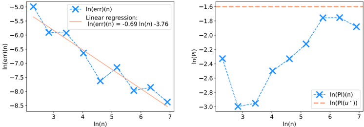
The image displays two side-by-side log-log plots. The left plot analyzes the natural logarithm of an error metric, `ln(err)(n)`, against the natural logarithm of a parameter `n`. The right plot analyzes the natural logarithm of a performance index, `ln(PI)(n)`, against the same `ln(n)`. Both plots use blue 'X' markers connected by dashed lines for the data series and include an orange reference line.
### Components/Axes
**Left Plot:**
* **Y-axis:** Label is `ln(err)(n)`. Scale ranges from approximately -8.5 to -5.0.
* **X-axis:** Label is `ln(n)`. Scale ranges from approximately 2.5 to 7.0.
* **Legend (Top-Right Corner):**
* Blue 'X' with dashed line: `ln(err)(n)`
* Solid orange line: `Linear regression: ln(err)(n) = -0.69 ln(n) - 3.76`
* **Data Series:** Blue 'X' markers connected by a blue dashed line.
* **Reference Line:** A solid orange line representing the linear regression fit.
**Right Plot:**
* **Y-axis:** Label is `ln(PI)`. Scale ranges from approximately -3.0 to -1.6.
* **X-axis:** Label is `ln(n)`. Scale ranges from approximately 2.5 to 7.0.
* **Legend (Bottom-Right Corner):**
* Blue 'X' with dashed line: `ln(PI)(n)`
* Dashed orange line: `ln(PI(u*))`
* **Data Series:** Blue 'X' markers connected by a blue dashed line.
* **Reference Line:** A horizontal dashed orange line.
### Detailed Analysis
**Left Plot - `ln(err)(n)` vs. `ln(n)`:**
* **Trend Verification:** The data series shows a clear downward trend. As `ln(n)` increases, `ln(err)(n)` generally decreases, indicating the error `err(n)` decreases as `n` increases.
* **Data Points (Approximate):**
* (ln(n) ≈ 2.5, ln(err) ≈ -5.0)
* (ln(n) ≈ 3.0, ln(err) ≈ -5.9)
* (ln(n) ≈ 3.5, ln(err) ≈ -5.9)
* (ln(n) ≈ 4.0, ln(err) ≈ -6.6)
* (ln(n) ≈ 4.5, ln(err) ≈ -7.6) *[Notable dip]*
* (ln(n) ≈ 5.0, ln(err) ≈ -7.1)
* (ln(n) ≈ 5.5, ln(err) ≈ -7.9)
* (ln(n) ≈ 6.0, ln(err) ≈ -8.0)
* (ln(n) ≈ 6.5, ln(err) ≈ -7.8)
* (ln(n) ≈ 7.0, ln(err) ≈ -8.4)
* **Linear Regression:** The fitted line has the equation `ln(err)(n) = -0.69 ln(n) - 3.76`. This implies a power-law relationship: `err(n) ≈ e^{-3.76} * n^{-0.69}`.
**Right Plot - `ln(PI)(n)` vs. `ln(n)`:**
* **Trend Verification:** The data series shows an initial drop followed by a general upward trend. `ln(PI)(n)` increases with `ln(n)` after the first point, suggesting the performance index `PI(n)` improves (increases) with larger `n`.
* **Data Points (Approximate):**
* (ln(n) ≈ 2.5, ln(PI) ≈ -2.4)
* (ln(n) ≈ 3.0, ln(PI) ≈ -3.0) *[Minimum]*
* (ln(n) ≈ 3.5, ln(PI) ≈ -2.9)
* (ln(n) ≈ 4.0, ln(PI) ≈ -2.5)
* (ln(n) ≈ 4.5, ln(PI) ≈ -2.3)
* (ln(n) ≈ 5.0, ln(PI) ≈ -2.1)
* (ln(n) ≈ 5.5, ln(PI) ≈ -1.7)
* (ln(n) ≈ 6.0, ln(PI) ≈ -1.7) *[Plateau/Maximum]*
* (ln(n) ≈ 6.5, ln(PI) ≈ -1.9)
* **Reference Line:** The horizontal dashed line `ln(PI(u*))` is positioned at approximately y = -1.6. This represents a constant, possibly optimal or asymptotic, value for the performance index.
### Key Observations
1. **Inverse Relationship (Left Plot):** There is a strong inverse relationship between `err(n)` and `n`, quantified by the negative slope (-0.69) of the regression line on the log-log scale.
2. **Non-Monotonic Behavior (Right Plot):** The performance index `PI(n)` does not improve monotonically. It worsens initially (from ln(n)=2.5 to 3.0) before beginning a sustained improvement.
3. **Convergence (Right Plot):** The data series `ln(PI)(n)` appears to approach, but not yet reach, the constant reference level `ln(PI(u*))` at the largest values of `ln(n)` shown (around 6.0-6.5).
4. **Outlier/Dip (Left Plot):** The data point at `ln(n) ≈ 4.5` shows a significantly lower error than the trend would predict, creating a noticeable dip in the series.
### Interpretation
These plots likely analyze the convergence behavior of a numerical method or algorithm as a problem size or resolution parameter `n` increases.
* **Left Plot (Error):** Demonstrates that the method is **convergent**, as the error decreases with increasing `n`. The power-law exponent of -0.69 suggests a sub-linear convergence rate (slower than 1/n). The dip at `ln(n)=4.5` could indicate a particularly favorable problem size or a numerical artifact.
* **Right Plot (Performance Index):** Suggests the method's **efficiency or quality** (PI) generally improves with scale but has a complex, non-monotonic relationship at smaller scales. The approach towards the horizontal line `ln(PI(u*))` indicates the performance may be saturating towards a fundamental limit `u*` as `n` grows very large. The initial drop implies a "start-up" cost or inefficiency at small `n`.
**Together, the plots tell a story:** As you invest more resources (increase `n`), your solution becomes more accurate (error drops), and its overall performance improves, eventually nearing a theoretical optimum, though the path to improvement isn't perfectly smooth. The analysis is conducted in log-log space to clearly reveal power-law relationships and orders of magnitude.