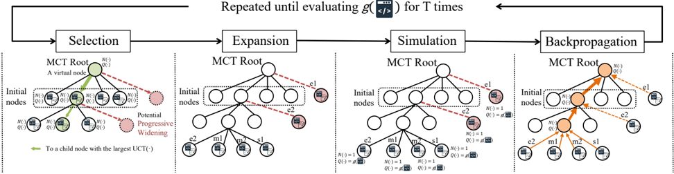
## Flowchart: Monte Carlo Tree Search (MCTS) Algorithm Phases
### Overview
The diagram illustrates the four iterative phases of the Monte Carlo Tree Search (MCTS) algorithm: **Selection**, **Expansion**, **Simulation**, and **Backpropagation**. These phases repeat until a terminal condition (evaluating `g(·)` for `T` times) is met. The flowchart uses color-coded arrows and nodes to represent decision-making and state transitions.
---
### Components/Axes
1. **Nodes**:
- **MCT Root**: Central virtual node (green circle) acting as the starting point.
- **Initial Nodes**: Pre-existing child nodes (white circles) with `N(·)` and `Q(·)` values.
- **Potential Progressive Widening**: Red dashed circles indicating unexplored nodes.
- **New Nodes**: Labeled `e1`, `e2`, `m1`, `m2`, `s1` (expanded during Simulation/Backpropagation).
2. **Arrows**:
- **Green**: "To a child node with the largest UCT(·)" (Selection phase).
- **Red**: "Potential Progressive Widening" (Selection phase).
- **Orange**: "Backpropagation" updates (Backpropagation phase).
3. **Legend**:
- **Colors**:
- Green: Selection actions.
- Red: Unexplored nodes.
- Orange: Backpropagation updates.
- **Placement**: Bottom-left corner.
4. **Text Labels**:
- **Selection**: "A virtual node", "To a child node with the largest UCT(·)".
- **Expansion**: "e1", "e2" (new nodes added).
- **Simulation**: "N(·)=1", "Q(·)=g(·)" (evaluation metrics).
- **Backpropagation**: "N(·)=1", "Q(·)=g(·)" (updated values).
---
### Detailed Analysis
1. **Selection Phase**:
- The MCT Root node evaluates child nodes using the **UCT formula** (Upper Confidence Bound applied to Trees).
- Green arrows direct selection to the child node with the highest UCT value.
- Red dashed circles represent unexplored nodes ("Potential Progressive Widening").
2. **Expansion Phase**:
- New nodes (`e1`, `e2`) are added to the tree, expanding the search space.
- Dashed lines connect the MCT Root to these nodes, indicating potential future paths.
3. **Simulation Phase**:
- Nodes are evaluated using a heuristic or simulation (`g(·)` function).
- `N(·)` and `Q(·)` values are initialized (e.g., `N(·)=1`, `Q(·)=g(·)`).
4. **Backpropagation Phase**:
- Results from Simulation propagate upward via orange arrows.
- The MCT Root and intermediate nodes update their `N(·)` and `Q(·)` values based on simulation outcomes.
---
### Key Observations
- **Iterative Process**: The flowchart emphasizes repetition until `g(·)` is evaluated `T` times, suggesting a loop structure.
- **Node Prioritization**: UCT values guide exploration-exploitation trade-offs during Selection.
- **Color Coding**: Distinct colors (green, red, orange) visually separate phases and actions.
- **Dashed vs. Solid Lines**: Dashed lines denote potential nodes; solid lines represent confirmed paths.
---
### Interpretation
The diagram demonstrates how MCTS balances exploration (trying new nodes) and exploitation (leveraging known high-value nodes). The UCT formula ensures efficient search by prioritizing nodes with high potential. The use of `N(·)` (visit count) and `Q(·)` (action value) tracks node performance, while backpropagation refines these estimates iteratively. The repetition until `T` evaluations implies a bounded computational budget, critical for real-time applications like game AI. The color-coded arrows and nodes simplify understanding of the algorithm’s flow, making it accessible for technical documentation.