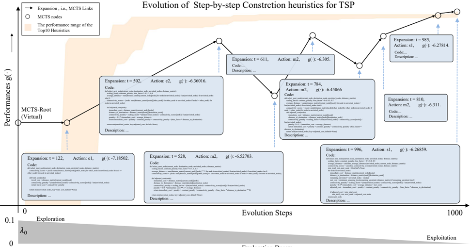
## Diagram: Evolution of Step-by-step Constriction heuristics for TSP ### Overview This image is a technical diagram illustrating the evolutionary process of heuristic algorithms for the Traveling Salesperson Problem (TSP). It visualizes a search or optimization trajectory, likely from a Monte Carlo Tree Search (MCTS) process, showing how different heuristic "actions" are applied at various "expansion" steps, leading to changes in performance. The diagram combines a flowchart of nodes and connections with embedded code snippets and performance metrics. ### Components/Axes * **Title:** "Evolution of Step-by-step Constriction heuristics for TSP" * **Y-Axis (Vertical):** Labeled "Performances g(·)". The scale runs from 0.1 at the bottom to 0 at the top. An upward-pointing arrow indicates the direction of increasing performance (i.e., values closer to 0 are better). * **X-Axis (Horizontal):** Labeled "Evolution Steps". The scale runs from 0 on the left to 1000 on the right. * **Legend (Top-Left):** * `→` : "Expansion, i.e., MCTS Links" * `○` : "MCTS nodes" * Shaded Orange Area: "The performance range of the Top10 Heuristics" * **Bottom Annotations:** * "Exploration" is labeled on the left side of the x-axis. * "Exploitation" is labeled on the right side of the x-axis. * A parameter `λ₀` is indicated near the origin (0,0). * **Node Structure:** Each node (circle) is connected by arrows (expansion links). Associated with most nodes is a rectangular box containing: * `Expansion: t = [Number],` * `Action: [e1, e2, m1, or m2],` * `g(·): [Negative Decimal Value],` * `Code: [Truncated code snippet]` * `Description: ...` (This field is empty or truncated in all visible boxes). ### Detailed Analysis The diagram traces a path from an initial virtual root node through a series of expansions. The performance `g(·)` generally improves (becomes less negative) as the evolution steps increase, though the path is not strictly monotonic. **Node-by-Node Data (from left to right along the evolutionary path):** 1. **MCTS-Root (Virtual):** Located at the far left (Step ~0). No data box is attached. It serves as the starting point. 2. **Node 1 (Bottom-Left):** * Expansion: t = 122 * Action: e1 * g(·): -7.18502 * Code: (Truncated) Begins with `#include <vector>...` and contains references to `constriction`, `distance`, `heuristic`, `solution`. 3. **Node 2 (Top-Left-Center):** * Expansion: t = 502 * Action: e2 * g(·): -6.36016 * Code: (Truncated) Similar structure to Node 1, with different parameter values. 4. **Node 3 (Bottom-Center):** * Expansion: t = 528 * Action: m2 * g(·): -6.52703 * Code: (Truncated) 5. **Node 4 (Top-Center):** * Expansion: t = 611 * Action: m2 * g(·): -6.305 * Code: (Truncated) 6. **Node 5 (Center-Right):** * Expansion: t = 784 * Action: m2 * g(·): -6.45066 * Code: (Truncated) 7. **Node 6 (Top-Right):** * Expansion: t = 810 * Action: m2 * g(·): -6.311 * Code: (Truncated) 8. **Node 7 (Bottom-Right):** * Expansion: t = 996 * Action: s1 * g(·): -6.26859 * Code: (Truncated) 9. **Node 8 (Top-Rightmost):** * Expansion: t = 985 * Action: s1 * g(·): -6.27814 * Code: (Truncated) **Visual Trend Verification:** * The overall trajectory of connected nodes moves from the bottom-left (lower performance) towards the top-right (higher performance). * The shaded orange "Top10 Heuristics" band occupies the upper portion of the graph, indicating the performance zone the evolving heuristics are approaching. * The path shows fluctuations. For example, performance improves from Node 1 (`g=-7.185`) to Node 2 (`g=-6.360`), then dips at Node 3 (`g=-6.527`), before improving again at Node 4 (`g=-6.305`). ### Key Observations 1. **Performance Improvement:** The primary trend is a clear improvement in the heuristic performance metric `g(·)`, moving from approximately -7.19 to -6.27 over ~1000 evolution steps. 2. **Action Types:** Four distinct action types are logged: `e1`, `e2`, `m1` (not observed in this path), `m2`, and `s1`. The later stages of the evolution (steps > 700) are dominated by `m2` and `s1` actions. 3. **Non-Monotonic Progress:** The search path is not a straight line to improvement. There are steps where performance temporarily decreases (e.g., from Node 2 to Node 3), suggesting exploration of potentially sub-optimal heuristics that may lead to better long-term solutions. 4. **Convergence Proximity:** The final nodes (7 and 8) have very similar performance values (`-6.26859` and `-6.27814`), suggesting the search may be converging near a local optimum within the "Top10" performance range. 5. **Code-Driven Evolution:** Each step is associated with a specific, generated code snippet for a constriction heuristic, indicating this is a programmatic or genetic programming approach to algorithm evolution. ### Interpretation This diagram visualizes the **exploratory search process** of an automated algorithm design system. It doesn't just show a final result; it maps the *history of discovery*. * **What it demonstrates:** The system starts with a basic heuristic (e1) and iteratively modifies it through actions (e2, m2, s1). Each modification is a hypothesis tested via expansion in the search tree (MCTS). The performance `g(·)` acts as the fitness signal. The shaded "Top10" band represents the known frontier of high-performing heuristics, which the evolutionary process successfully navigates toward. * **Relationship between elements:** The **nodes** are specific heuristic implementations (code). The **arrows** represent the decision to explore a variation of a parent heuristic. The **x-axis (Steps)** is the computational budget or time. The **y-axis (Performance)** is the objective function being maximized (minimized, as g(·) is negative). * **Notable Insight:** The path reveals that the most significant performance jump occurs early (from step 122 to 502). Later improvements are more incremental, which is characteristic of optimization processes where easy gains are found first, followed by fine-tuning. The presence of `s1` actions in the final steps suggests a shift to a different, possibly more refined, modification strategy as the search matures. The diagram effectively argues for the efficacy of this step-by-step, code-generating evolutionary approach by showing its trajectory into the elite performance zone.