## Diagram: Coordinate Grid with Boundary Margin
### Overview
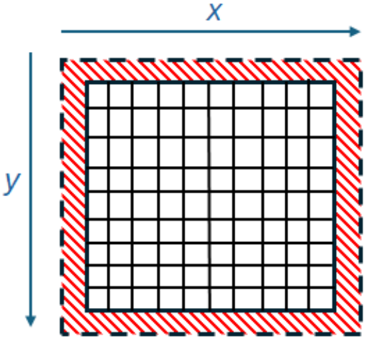
The image is a technical diagram illustrating a two-dimensional grid system with a defined boundary margin. It depicts a Cartesian coordinate system with a central grid area surrounded by a striped border region, likely representing a margin, buffer zone, or area of exclusion.
### Components/Axes
* **Coordinate Axes:**
* **Horizontal Axis (x):** Located at the top of the diagram. A blue arrow points to the right, labeled with the variable **"x"**.
* **Vertical Axis (y):** Located on the left side of the diagram. A blue arrow points downward, labeled with the variable **"y"**.
* **Central Grid:** A square region composed of a 10x10 array of smaller, empty white squares defined by black grid lines.
* **Boundary Margin:** A border region surrounding the central grid on all four sides. It is filled with a pattern of diagonal red and white stripes (hatching). The outer edge of this margin is defined by a dashed black line.
### Detailed Analysis
* **Grid Structure:** The central grid is a perfect square, subdivided into 100 smaller cells (10 columns by 10 rows).
* **Margin Dimensions:** The striped margin appears to be of uniform thickness around the entire grid. Visually, its width is approximately equal to the side length of one small grid cell.
* **Spatial Relationships:**
* The **x-axis** arrow is positioned above the top edge of the margin.
* The **y-axis** arrow is positioned to the left of the left edge of the margin.
* The **dashed black line** forms the outermost boundary of the entire figure.
* The **striped margin** lies between the dashed outer boundary and the solid black lines of the inner grid.
* The **inner grid** is centered within the margin.
### Key Observations
1. **Directional Indicators:** The arrows on the axes explicitly define the positive directions for the coordinate system: right for `x` and down for `y`. This is a common convention in computer graphics and matrix indexing.
2. **Boundary Definition:** The diagram clearly distinguishes between two zones: an "inner" active grid area and an "outer" margin or boundary zone, highlighted by the distinct striped pattern.
3. **Precision:** The grid is drawn with precise, straight lines, indicating a mathematical or computational model rather than a freehand sketch.
### Interpretation
This diagram is a foundational schematic for concepts involving bounded 2D spaces. It visually communicates several key technical ideas:
* **Coordinate System:** It establishes a reference frame (`x`, `y`) for locating points within the grid.
* **Domain vs. Boundary:** The core concept is the separation of a primary computational or data domain (the inner grid) from a surrounding boundary region (the striped margin). This is critical in fields like numerical analysis (e.g., finite difference methods, where boundary conditions are applied), image processing (e.g., padding for convolution), and game development (e.g., defining a play area with a buffer zone).
* **Margin Function:** The striped pattern suggests this area is special—it might be where boundary conditions are enforced, where data is padded or mirrored, or an area that is excluded from certain operations. The uniformity of the margin implies a consistent rule applied to all edges.
* **Visual Abstraction:** The lack of specific numerical values on the axes or grid makes this a generic template. It can represent any discretized 2D space, from a pixel array to a spatial simulation grid. The viewer is meant to understand the *relationship* between the components rather than specific measurements.
**In summary, the image provides a clear, abstract representation of a 2D grid with a defined boundary margin, serving as a visual reference for technical discussions about spatial domains, coordinate systems, and boundary conditions.**