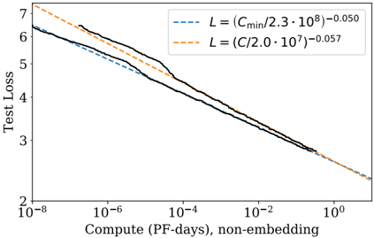
## Line Graph: Test Loss vs Compute (PF-days), non-embedding ### Overview The image depicts a logarithmic-scale line graph comparing two test loss functions (L) against compute resources (PF-days) for non-embedding tasks. Two distinct loss functions are visualized: one based on `C_min` and another on `C`, with differing exponents and constants. The graph shows how test loss decreases as compute increases, with both lines converging at higher compute values. ### Components/Axes - **Y-axis (Test Loss)**: Logarithmic scale ranging from 2 to 7. - **X-axis (Compute, PF-days, non-embedding)**: Logarithmic scale from 10⁻⁸ to 10⁰. - **Legend**: Located in the top-right corner, containing: - **Blue dashed line**: `L = (C_min/2.3·10⁸)⁻⁰·⁰⁵⁰` - **Orange dashed line**: `L = (C/2.0·10⁷)⁻⁰·⁰⁵⁷` ### Detailed Analysis 1. **Blue Dashed Line (`C_min`)**: - Starts at ~6.5 test loss at 10⁻⁸ PF-days. - Decreases steeply, reaching ~3.5 at 10⁻² PF-days. - Continues declining to ~2.5 at 10⁰ PF-days. - Equation suggests sensitivity to `C_min` with a weaker exponent (-0.050). 2. **Orange Dashed Line (`C`)**: - Begins at ~7 test loss at 10⁻⁸ PF-days. - Declines more gradually than the blue line, reaching ~3.0 at 10⁻² PF-days. - Converges with the blue line near 10⁻⁴ PF-days, then follows a similar trajectory. - Equation indicates higher sensitivity to `C` with a steeper exponent (-0.057). 3. **Convergence Point**: - Both lines intersect near 10⁻⁴ PF-days (~0.0001 PF-days). - Beyond this point, the lines overlap almost perfectly, suggesting diminishing differences in loss function performance at higher compute levels. ### Key Observations - **Initial Divergence**: The blue line (`C_min`) starts lower but decreases faster initially, while the orange line (`C`) begins higher but declines more slowly. - **Logarithmic Scaling**: The x-axis compression emphasizes performance differences at low compute levels (10⁻⁸ to 10⁻⁴ PF-days). - **Exponent Impact**: The steeper exponent (-0.057) for `C` amplifies its sensitivity to compute increases compared to `C_min` (-0.050). ### Interpretation The graph demonstrates that both loss functions improve with increased compute, but their efficiency profiles differ: - **`C_min`** (blue) is more effective at low compute levels, achieving lower loss faster. - **`C`** (orange) requires more compute to match `C_min`’s performance but becomes equally effective at higher compute levels (post-10⁻⁴ PF-days). - The convergence implies that optimizing for either loss function becomes equally viable beyond a critical compute threshold (~0.0001 PF-days). This suggests trade-offs in resource allocation: `C_min` may be preferable for constrained compute, while `C` could be better for scalable, high-resource scenarios.