## Diagram: Reasoning Model Architectures
### Overview
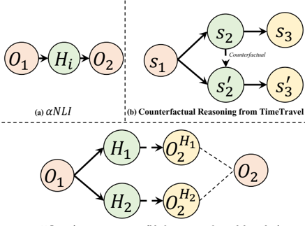
The image displays three distinct directed graph diagrams illustrating different reasoning or inference models. The diagrams are arranged in a two-row layout. The top row contains two side-by-side diagrams labeled (a) and (b). The bottom row contains a single, larger diagram. All diagrams use nodes (circles) containing text labels and directed edges (arrows) to represent relationships or flows between states or observations.
### Components/Axes
The image is a technical diagram with no traditional chart axes. The components are nodes and edges.
**Node Types & Labels:**
* **Observation Nodes (Pink):** Labeled `O₁`, `O₂`, `O₂^{H₁}`, `O₂^{H₂}`.
* **Hypothesis/State Nodes (Green):** Labeled `Hᵢ`, `H₁`, `H₂`, `s₁`, `s₂`, `s₂'`.
* **State/Outcome Nodes (Yellow):** Labeled `s₃`, `s₃'`.
**Diagram Labels & Titles:**
* **(a) αNLI:** Located below the top-left diagram.
* **(b) Counterfactual Reasoning from TimeTravel:** Located below the top-right diagram.
* **Bottom Diagram:** No explicit title is visible within the cropped image frame.
**Spatial Layout:**
* **Top-Left (a):** A linear chain: `O₁` → `Hᵢ` → `O₂`.
* **Top-Right (b):** A branching structure from `s₁` to two parallel paths (`s₂`→`s₃` and `s₂'`→`s₃'`), with a dashed arrow labeled "Counterfactual" connecting `s₂` to `s₂'`.
* **Bottom:** A branching and converging structure. `O₁` branches to `H₁` and `H₂`. Each `H` node points to a corresponding `O` node (`O₂^{H₁}` and `O₂^{H₂}`). Both `O₂^{H₁}` and `O₂^{H₂}` have dashed arrows pointing to a final `O₂` node.
### Detailed Analysis
**Diagram (a) αNLI:**
* **Structure:** A simple, linear, three-node chain.
* **Flow:** `O₁` (Observation 1) leads to `Hᵢ` (Hypothesis i), which in turn leads to `O₂` (Observation 2).
* **Interpretation:** This represents a basic abductive or inference model where an initial observation suggests a hypothesis, which then explains or predicts a subsequent observation.
**Diagram (b) Counterfactual Reasoning from TimeTravel:**
* **Structure:** A branching path from a single starting state.
* **Flow:** `s₁` (State 1) branches into two paths:
1. **Factual Path:** `s₁` → `s₂` → `s₃`.
2. **Counterfactual Path:** `s₁` → `s₂'` → `s₃'`.
* **Key Relationship:** A dashed arrow labeled "Counterfactual" connects `s₂` to `s₂'`, indicating that `s₂'` is a counterfactual alternative to `s₂`.
* **Interpretation:** This models reasoning about alternative scenarios. Starting from a common state `s₁`, it explores what would happen (`s₂'`, `s₃'`) if a different choice or event (`s₂'` instead of `s₂`) had occurred.
**Bottom Diagram (Unlabeled):**
* **Structure:** A branching-then-converging structure.
* **Flow:**
1. **Branching:** `O₁` leads to two competing hypotheses, `H₁` and `H₂`.
2. **Prediction:** Each hypothesis generates its own predicted observation: `H₁` → `O₂^{H₁}` and `H₂` → `O₂^{H₂}`.
3. **Convergence:** Both predicted observations (`O₂^{H₁}` and `O₂^{H₂}`) point via dashed arrows to a single, final observed outcome `O₂`.
* **Interpretation:** This represents a model for evaluating multiple hypotheses against a single observed outcome. The dashed lines suggest a comparison or evaluation step where the predictions from `H₁` and `H₂` are checked against the actual `O₂`.
### Key Observations
1. **Visual Coding:** Nodes are consistently color-coded by type across all diagrams: Pink for Observations (`O`), Green for Hypotheses/States (`H`, `s`), and Yellow for subsequent States/Outcomes (`s`).
2. **Edge Semantics:** Solid arrows represent direct causal or inferential flow. Dashed arrows represent a different relationship: a counterfactual link in (b) and a comparison/evaluation link in the bottom diagram.
3. **Complexity Progression:** The diagrams show increasing structural complexity from the linear chain (a), to the branching counterfactual (b), to the branching-and-converging hypothesis evaluation (bottom).
4. **Notation:** Subscripts (`₁`, `₂`, `₃`, `i`) denote sequence or instance. Superscripts (`^{H₁}`, `^{H₂}`) denote dependency or origin (e.g., `O₂` as predicted by `H₁`).
### Interpretation
This image succinctly illustrates three fundamental paradigms in computational reasoning and inference:
1. **Abductive Reasoning (αNLI):** The simplest model, inferring the most plausible hypothesis (`Hᵢ`) that explains a sequence of observations (`O₁`, `O₂`). This is core to tasks like Natural Language Inference (NLI).
2. **Counterfactual Reasoning:** A more sophisticated model that asks "what if?" It requires maintaining parallel world models (the factual `s₂→s₃` and the counterfactual `s₂'→s₃'`) and understanding the minimal change that differentiates them. This is crucial for causal analysis and planning.
3. **Hypothesis Discrimination/Evaluation:** The bottom diagram models a scientific or diagnostic process. Given an initial observation (`O₁`), multiple hypotheses (`H₁`, `H₂`) are generated. Each makes a testable prediction (`O₂^{H₁}`, `O₂^{H₂}`). The actual outcome (`O₂`) is then used to evaluate which hypothesis's prediction was more accurate, thereby supporting or falsifying the hypotheses.
The progression suggests a hierarchy of reasoning capabilities, from simple explanation to complex evaluation of alternatives against evidence. The consistent visual language (color, node labels, edge styles) allows for direct comparison of the underlying logical structures of these different reasoning tasks.