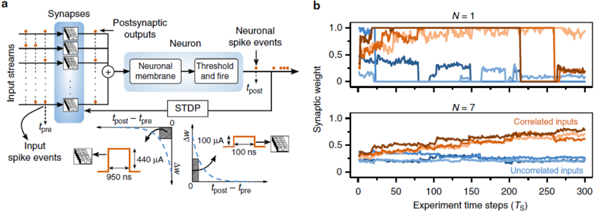
## Diagram and Charts: Neuromorphic Synaptic Plasticity System ### Overview The image is a two-part technical figure illustrating a neuromorphic computing system that implements Spike-Timing-Dependent Plasticity (STDP). Part (a) is a schematic diagram of the system architecture and learning rule. Part (b) presents two line charts showing experimental results of synaptic weight evolution over time under different input conditions. ### Components/Axes **Part (a) - System Diagram:** * **Left Section (Input & Synapses):** Labeled "Input streams" (vertical lines with dots representing "Input spike events"). These connect to a block labeled "Synapses" (blue shaded area containing three stacked synaptic device symbols). A timing diagram shows a pre-synaptic pulse with a width of "950 ns" and amplitude of "440 µA". * **Center Section (Neuron):** A summation symbol (⊕) receives "Postsynaptic outputs" from the synapses. This feeds into a "Neuron" block containing "Neuronal membrane" and "Threshold and fire" sub-blocks. The output is labeled "Neuronal spike events" at time `t_post`. * **Feedback Loop (STDP):** A block labeled "STDP" receives inputs from the pre-synaptic spike time (`t_pre`) and the post-synaptic spike time (`t_post`). It outputs a weight change (`ΔW`) based on the timing difference `t_post - t_pre`. Two timing diagrams illustrate the STDP function: * Left: A post-before-pre spike pair (`t_post - t_pre < 0`) leads to a negative `ΔW` (depression). The pulse width is "100 ns" and amplitude is "100 µA". * Right: A pre-before-post spike pair (`t_post - t_pre > 0`) leads to a positive `ΔW` (potentiation). * **Labels:** `t_pre`, `t_post`, `t_post - t_pre`, `ΔW`. **Part (b) - Experimental Charts:** * **Top Chart (N = 1):** * **Y-axis:** "Synaptic weight" (scale: 0 to 1.0, with ticks at 0, 0.5, 1.0). * **X-axis:** Not explicitly labeled, but implied to be time steps, consistent with the bottom chart. * **Data Series:** Three lines (orange, dark blue, light blue). No legend is present in this specific chart. * **Bottom Chart (N = 7):** * **Y-axis:** "Synaptic weight" (scale: 0 to 1.0, with ticks at 0, 0.5, 1.0). * **X-axis:** "Experiment time steps (Ts)" (scale: 0 to 300, with ticks every 50 units). * **Legend:** Located in the top-right corner of the chart area. * Orange line: "Correlated inputs" * Blue line: "Uncorrelated inputs" * **Data Series:** Two primary lines (orange and blue), each with a shaded region (likely representing standard deviation or error across multiple trials). ### Detailed Analysis **Part (a) - Diagram Flow:** The system operates as follows: 1. Multiple input spike streams are received by a layer of synaptic devices. 2. The synaptic outputs are summed and fed into a neuron circuit. 3. The neuron integrates the input, and when a threshold is reached, it fires a post-synaptic spike (`t_post`). 4. The STDP learning circuit compares the timing of pre-synaptic (`t_pre`) and post-synaptic (`t_post`) spikes. 5. Based on this timing difference (`t_post - t_pre`), it generates a weight change signal (`ΔW`) to update the synaptic devices, implementing Hebbian learning. **Part (b) - Chart Data & Trends:** * **Top Chart (N = 1 - Single Synapse):** * **Orange Line Trend:** Starts high (~0.8-0.9), exhibits high volatility with large, rapid fluctuations between ~0.2 and 1.0 throughout the time series. It shows no clear long-term increasing or decreasing trend. * **Dark Blue Line Trend:** Starts moderately high (~0.7), experiences a sharp, significant drop to near 0 around time step ~25. It then partially recovers to ~0.4 and fluctuates in the 0.2-0.5 range for the remainder of the experiment. * **Light Blue Line Trend:** Starts low (~0.2), remains relatively stable with minor fluctuations between ~0.1 and 0.3 for the entire duration. * **Bottom Chart (N = 7 - Seven Synapses):** * **Orange Line (Correlated inputs) Trend:** Shows a clear, steady upward trend. It starts at a synaptic weight of ~0.3 and increases to approximately 0.7-0.8 by time step 300. The shaded region indicates moderate variance across trials. * **Blue Line (Uncorrelated inputs) Trend:** Remains essentially flat. It starts at ~0.3 and stays within the 0.2-0.4 range for the entire experiment, showing no significant potentiation or depression. The shaded region is narrower than for the correlated case. ### Key Observations 1. **Learning Rule Implementation:** The diagram in (a) successfully depicts a complete closed-loop STDP system, from spike sensing to weight update. 2. **Volatility vs. Stability:** The single synapse (N=1) data is highly volatile and unstable, while the averaged data from seven synapses (N=7) shows smooth, clear trends. 3. **Correlation-Driven Plasticity:** The most significant finding is in the N=7 chart. Synapses receiving **correlated inputs** undergo strong, consistent potentiation (weight increase). Synapses receiving **uncorrelated inputs** show no significant change in weight. 4. **Color Consistency:** The orange color is consistently used for the "Correlated inputs" series in the bottom chart's legend and data line. The blue color is used for "Uncorrelated inputs." ### Interpretation This figure demonstrates the fundamental principle of Hebbian learning ("neurons that fire together, wire together") in a hardware-implemented neuromorphic system. * **What the data suggests:** The system successfully learns to strengthen synaptic connections that contribute to causing the post-synaptic neuron to fire (correlated activity). Synapses that are not causally related to the output (uncorrelated) do not strengthen and may even weaken slightly relative to the potentiated ones. This is the core mechanism for pattern recognition and memory formation in biological and artificial neural networks. * **How elements relate:** The diagram (a) explains the *mechanism* (STDP), while the charts (b) provide the *empirical evidence* of its function. The transition from the noisy, single-device behavior (N=1) to the clean, averaged behavior (N=7) highlights the importance of population coding and averaging in extracting reliable signals from inherently stochastic neuromorphic components. * **Notable anomalies:** The dramatic drop in the dark blue line in the N=1 chart is an outlier event, possibly representing a potentiation-to-depression transition or a device-specific instability. The fact that the uncorrelated (blue) line in the N=7 chart does not decay to zero suggests a baseline maintenance mechanism or a lower bound on the weight. * **Broader significance:** This validates the use of nanoscale synaptic devices (like memristors) for on-chip, unsupervised learning. The clear separation between correlated and uncorrelated input responses shows the system can discriminate and encode temporal patterns, which is essential for processing real-world sensory data like audio or video.