## Bar Chart: RMSE vs. Averaging Period
### Overview
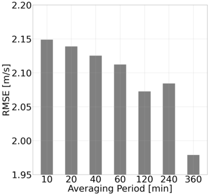
The image is a vertical bar chart displaying the Root Mean Square Error (RMSE) in meters per second (m/s) as a function of different averaging periods in minutes. The chart illustrates how the error metric changes as the time window for averaging data increases.
### Components/Axes
* **X-Axis (Horizontal):** Labeled "Averaging Period [min]". It contains seven categorical bars corresponding to the following discrete time periods: 10, 20, 40, 60, 120, 240, and 360 minutes.
* **Y-Axis (Vertical):** Labeled "RMSE [m/s]". The scale is linear, ranging from a minimum of 1.95 to a maximum of 2.20, with major gridlines at intervals of 0.05 (1.95, 2.00, 2.05, 2.10, 2.15, 2.20).
* **Data Series:** A single series represented by solid gray bars. There is no legend, as only one data type is plotted.
* **Spatial Layout:** The chart has a white background with light gray gridlines. The axes labels are positioned conventionally: the x-axis label is centered below the axis, and the y-axis label is rotated 90 degrees and placed to the left of the axis.
### Detailed Analysis
The following table reconstructs the approximate RMSE values for each averaging period, derived from visual inspection of the bar heights against the y-axis scale. The values are approximate, with an estimated uncertainty of ±0.01 m/s.
| Averaging Period (min) | Approximate RMSE (m/s) | Visual Trend Description |
| :--- | :--- | :--- |
| 10 | 2.15 | The tallest bar, representing the highest error. |
| 20 | 2.14 | Slightly shorter than the 10-minute bar. |
| 40 | 2.125 | Noticeably shorter than the 20-minute bar. |
| 60 | 2.11 | Continues the downward trend. |
| 120 | 2.07 | A significant drop from the 60-minute value. |
| 240 | 2.08 | **Anomaly:** Slightly taller than the 120-minute bar, breaking the consistent downward trend. |
| 360 | 1.98 | The shortest bar, representing the lowest error by a substantial margin. |
**Trend Verification:** The overall visual trend is a clear downward slope from left to right, indicating that RMSE generally decreases as the averaging period increases. The bar for 240 minutes is a minor exception to this monotonic decrease.
### Key Observations
1. **General Inverse Relationship:** There is a strong inverse relationship between averaging period and RMSE. Longer averaging periods are associated with lower error values.
2. **Non-Monotonic Point:** The data point at 240 minutes (RMSE ≈ 2.08 m/s) is slightly higher than the point at 120 minutes (RMSE ≈ 2.07 m/s), creating a small "bump" in the otherwise descending trend.
3. **Significant Final Drop:** The most substantial reduction in RMSE occurs between the 240-minute and 360-minute periods, where the error drops by approximately 0.10 m/s.
4. **Range of Variation:** The RMSE values span a range of approximately 0.17 m/s, from a high of ~2.15 m/s (10 min) to a low of ~1.98 m/s (360 min).
### Interpretation
This chart demonstrates the effect of temporal data aggregation on model or measurement error. The primary finding is that **increasing the averaging period reduces the RMSE**. This is a common pattern in signal processing and forecasting, where averaging over longer windows smooths out high-frequency noise and random fluctuations, leading to a more stable and accurate estimate (lower error).
The anomaly at 240 minutes is noteworthy. It suggests that the relationship is not perfectly linear or that other factors may influence the error at that specific time scale. It could be an artifact of the specific dataset, indicating a periodic signal or noise component with a cycle that interacts with the 4-hour (240-minute) averaging window, slightly degrading performance compared to the 2-hour window.
The dramatic improvement at 360 minutes (6 hours) implies that this longer period is particularly effective at filtering out the dominant sources of error in this context. The data strongly suggests that for this specific application, using an averaging period of 6 hours yields the most accurate results among the tested options. The choice of an optimal averaging period involves a trade-off: longer periods reduce noise but may also smooth out important short-term variations or introduce lag in a real-time system.