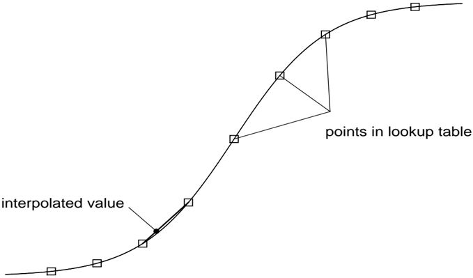
## Diagram: Interpolation from a Lookup Table ### Overview The image is a technical diagram illustrating the concept of interpolation using a lookup table. It depicts a smooth, continuous curve with discrete data points marked along it, and demonstrates how a value between two known points can be estimated. ### Components/Axes * **Main Element:** A single, smooth, S-shaped (sigmoidal) curve that rises from the lower-left to the upper-right of the frame. * **Data Points:** Twelve small, hollow square markers are placed at intervals along the curve. These represent known data points. * **Labels & Annotations:** * **"points in lookup table"**: This text is positioned in the center-right area of the image. Three thin lines extend from this label, each pointing to a different square marker on the upper half of the curve. This explicitly identifies those squares as the discrete entries stored in a lookup table. * **"interpolated value"**: This text is positioned in the lower-left area. A single thin line extends from this label, pointing to a small, solid black dot located on the curve *between* two of the square markers. This dot represents the estimated value derived through interpolation. * **Spatial Layout:** The diagram is minimal, with no axes, grids, or scales. The focus is solely on the relationship between the continuous curve, the discrete lookup points, and the interpolated point. ### Detailed Analysis * **Curve Trajectory:** The curve begins with a shallow slope in the bottom-left, steepens in the middle, and then flattens again towards the top-right. * **Point Distribution:** The square markers are not perfectly evenly spaced along the curve's length. The spacing appears slightly wider in the flatter regions (beginning and end) and narrower in the steeper central region. * **Interpolation Demonstration:** The solid black dot (interpolated value) is placed on the curve segment between the 4th and 5th square markers (counting from the bottom-left). A short, thick line segment is drawn on the curve connecting these two squares, visually emphasizing the interval over which the interpolation is performed. The black dot lies on this segment. ### Key Observations 1. **Conceptual, Not Quantitative:** The diagram is purely conceptual. It contains no numerical data, axis labels, units, or scales. Its purpose is to illustrate a method, not to present specific data. 2. **Visual Hierarchy:** The use of hollow squares for known points and a solid dot for the unknown, interpolated point creates a clear visual distinction between stored data and calculated results. 3. **Flow of Information:** The diagram implies a process: known values (squares) are stored in a lookup table. To find a value for an input not in the table, one locates the nearest known points and interpolates along the curve connecting them (the black dot). ### Interpretation This diagram serves as a fundamental visual explanation of **linear or curve-based interpolation**. It demonstrates how a continuous function or relationship (the smooth curve) can be approximated using a finite set of known data points (the lookup table). The "interpolated value" is the estimated output for an input that falls between two stored entries. The underlying message is about **efficiency and approximation**. Instead of storing an infinite number of points to define the curve, a system can store a manageable set of key points and use interpolation to estimate values in between. This is a core concept in computer graphics (e.g., texture mapping, animation), data analysis, signal processing, and numerical methods. The diagram effectively communicates the relationship between discrete data and continuous estimation without relying on complex mathematics.