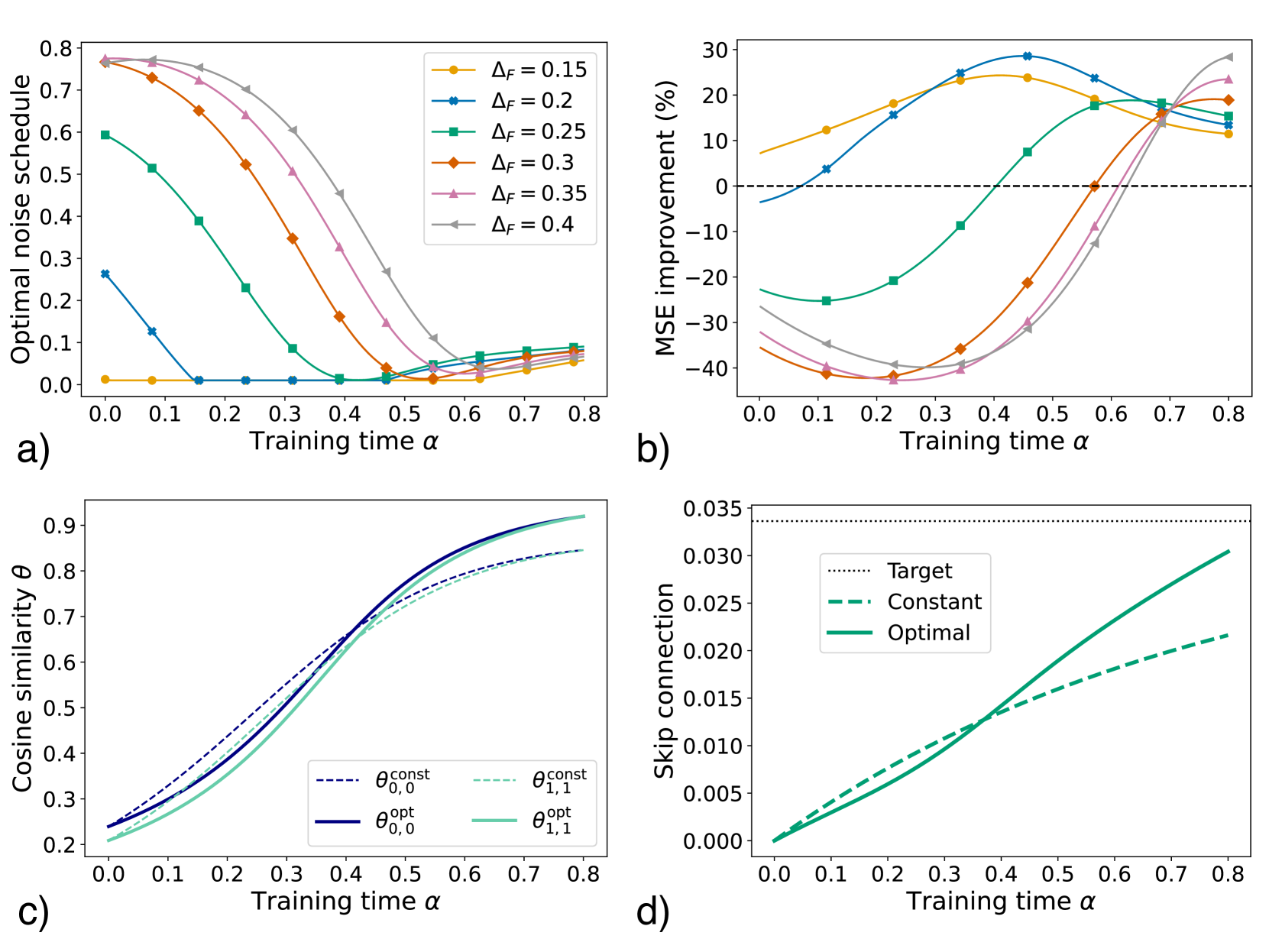
\n ## Multi-Panel Line Chart: Training Dynamics Analysis ### Overview The image is a composite figure containing four distinct line charts, labeled a), b), c), and d). Each chart plots a different performance or model parameter metric against a common x-axis variable, "Training time α". The charts collectively analyze the effects of a parameter ΔF and different optimization strategies (constant vs. optimal) on model training dynamics. ### Components/Axes * **Common X-Axis (All Panels):** "Training time α". The scale runs from 0.0 to 0.8 with major tick marks at 0.1 intervals. * **Panel a) Y-Axis:** "Optimal noise schedule". Scale from 0.0 to 0.8. * **Panel b) Y-Axis:** "MSE improvement (%)". Scale from -40 to 30. A horizontal dashed line at 0% indicates the baseline. * **Panel c) Y-Axis:** "Cosine similarity θ". Scale from 0.2 to 0.9. * **Panel d) Y-Axis:** "Skip connection". Scale from 0.000 to 0.035. * **Legends:** * **Panel a) & b):** Located in the top-right corner. Contains six entries for different values of ΔF: 0.15 (yellow circle), 0.2 (blue star), 0.25 (green square), 0.3 (orange diamond), 0.35 (pink triangle up), 0.4 (grey triangle down). * **Panel c):** Located in the bottom-right corner. Contains four entries: θ₀,₀^const (dark blue dashed line), θ₁,₁^const (light green dashed line), θ₀,₀^opt (dark blue solid line), θ₁,₁^opt (light green solid line). * **Panel d):** Located in the top-left corner. Contains three entries: Target (black dotted line), Constant (green dash-dot line), Optimal (green solid line). ### Detailed Analysis **Panel a) Optimal noise schedule vs. Training time α** * **Trend:** For all ΔF values, the optimal noise schedule decreases as training time α increases. The rate of decrease is steeper for higher ΔF values. * **Data Points (Approximate):** * **ΔF = 0.15 (Yellow):** Starts near 0.0 at α=0.0, remains near 0.0 until α≈0.6, then rises slightly to ~0.05 at α=0.8. * **ΔF = 0.2 (Blue):** Starts at ~0.26 at α=0.0, drops sharply to near 0.0 by α=0.15, and remains near 0.0. * **ΔF = 0.25 (Green):** Starts at ~0.60 at α=0.0, decreases steadily, crossing 0.1 at α≈0.35, and approaches 0.0 by α=0.5. * **ΔF = 0.3 (Orange):** Starts at ~0.77 at α=0.0, decreases, crossing 0.4 at α≈0.25 and 0.1 at α≈0.45. * **ΔF = 0.35 (Pink):** Starts at ~0.78 at α=0.0, follows a similar but slightly higher path than ΔF=0.3. * **ΔF = 0.4 (Grey):** Starts at ~0.78 at α=0.0, is the highest curve, crossing 0.4 at α≈0.4 and 0.1 at α≈0.55. **Panel b) MSE improvement (%) vs. Training time α** * **Trend:** The relationship is non-monotonic. For lower ΔF (0.15, 0.2), MSE improvement starts positive, peaks, then declines. For higher ΔF (0.25-0.4), improvement starts negative (worse than baseline), reaches a minimum, then rises sharply, often surpassing the lower ΔF curves at later training times (α > 0.6). * **Data Points (Approximate):** * **ΔF = 0.15 (Yellow):** Starts at ~7%, peaks at ~24% near α=0.45, declines to ~11% at α=0.8. * **ΔF = 0.2 (Blue):** Starts at ~-4%, rises to a peak of ~29% near α=0.45, declines to ~15% at α=0.8. * **ΔF = 0.25 (Green):** Starts at ~-23%, reaches a minimum of ~-25% near α=0.1, then rises, crossing 0% at α≈0.5 and reaching ~18% at α=0.8. * **ΔF = 0.3 (Orange):** Starts at ~-35%, reaches a minimum of ~-42% near α=0.2, then rises steeply, crossing 0% at α≈0.57 and reaching ~19% at α=0.8. * **ΔF = 0.35 (Pink):** Starts at ~-32%, minimum of ~-43% near α=0.25, crosses 0% at α≈0.62, reaches ~23% at α=0.8. * **ΔF = 0.4 (Grey):** Starts at ~-27%, minimum of ~-40% near α=0.25, crosses 0% at α≈0.65, reaches ~28% at α=0.8. **Panel c) Cosine similarity θ vs. Training time α** * **Trend:** All four curves show a steady, sigmoidal increase in cosine similarity as training time α increases. The "optimal" (opt) strategies consistently achieve higher similarity than their "constant" (const) counterparts for the same θ index. * **Data Points (Approximate):** * **θ₀,₀^const (Dark Blue Dashed):** Starts at ~0.24 at α=0.0, rises to ~0.85 at α=0.8. * **θ₁,₁^const (Light Green Dashed):** Starts at ~0.21 at α=0.0, rises to ~0.85 at α=0.8. * **θ₀,₀^opt (Dark Blue Solid):** Starts at ~0.24 at α=0.0, rises more steeply, reaching ~0.92 at α=0.8. * **θ₁,₁^opt (Light Green Solid):** Starts at ~0.21 at α=0.0, follows a path very close to θ₀,₀^opt, also reaching ~0.92 at α=0.8. **Panel d) Skip connection vs. Training time α** * **Trend:** The "Constant" and "Optimal" skip connection values increase linearly with training time α. The "Optimal" line has a steeper slope. The "Target" is a fixed horizontal line. * **Data Points (Approximate):** * **Target (Black Dotted):** Constant value of ~0.034 across all α. * **Constant (Green Dash-Dot):** Starts at 0.0 at α=0.0, increases linearly to ~0.022 at α=0.8. * **Optimal (Green Solid):** Starts at 0.0 at α=0.0, increases linearly with a steeper slope, reaching ~0.031 at α=0.8, approaching but not yet reaching the Target. ### Key Observations 1. **Trade-off in Panel b):** There is a clear trade-off between early-stage and late-stage performance. High ΔF values cause severe initial performance degradation (large negative MSE improvement) but lead to greater potential gains later in training. 2. **Convergence in Panel a):** Regardless of starting point, the optimal noise schedule for all ΔF values converges toward zero as training progresses (α > 0.6). 3. **Superiority of Optimal Strategies:** In both panels c) and d), the "opt" (optimal) strategies outperform their "const" (constant) counterparts, achieving higher cosine similarity and a faster approach to the target skip connection value. 4. **Crossover Point:** In panel b), a notable crossover occurs around α=0.65-0.7, where the initially poor-performing high-ΔF models begin to surpass the initially better low-ΔF models in MSE improvement. ### Interpretation This figure likely analyzes training dynamics in a machine learning context, possibly for diffusion models or neural networks with skip connections. The parameter ΔF appears to control a noise or perturbation schedule. * **Panels a) & b) together** suggest that a more aggressive initial noise schedule (high ΔF) is detrimental in the short term but beneficial for long-term model performance. The optimal strategy adapts this schedule, reducing noise as training stabilizes. * **Panel c)** demonstrates that adaptive ("optimal") training strategies lead to better alignment (higher cosine similarity) between model components or representations compared to fixed ("constant") strategies. * **Panel d)** shows that an adaptive approach for a skip connection parameter allows it to grow more efficiently toward a predefined target value, which is a common technique for stabilizing deep network training. **Overall Narrative:** The data argues for the use of adaptive, time-varying training schedules (for noise and skip connections) over fixed ones. While aggressive adaptive schedules may incur an initial performance cost, they facilitate superior final model alignment and performance, as evidenced by higher late-stage MSE improvement and cosine similarity. The charts provide a quantitative basis for designing such schedules by showing the evolution of key metrics over training time.