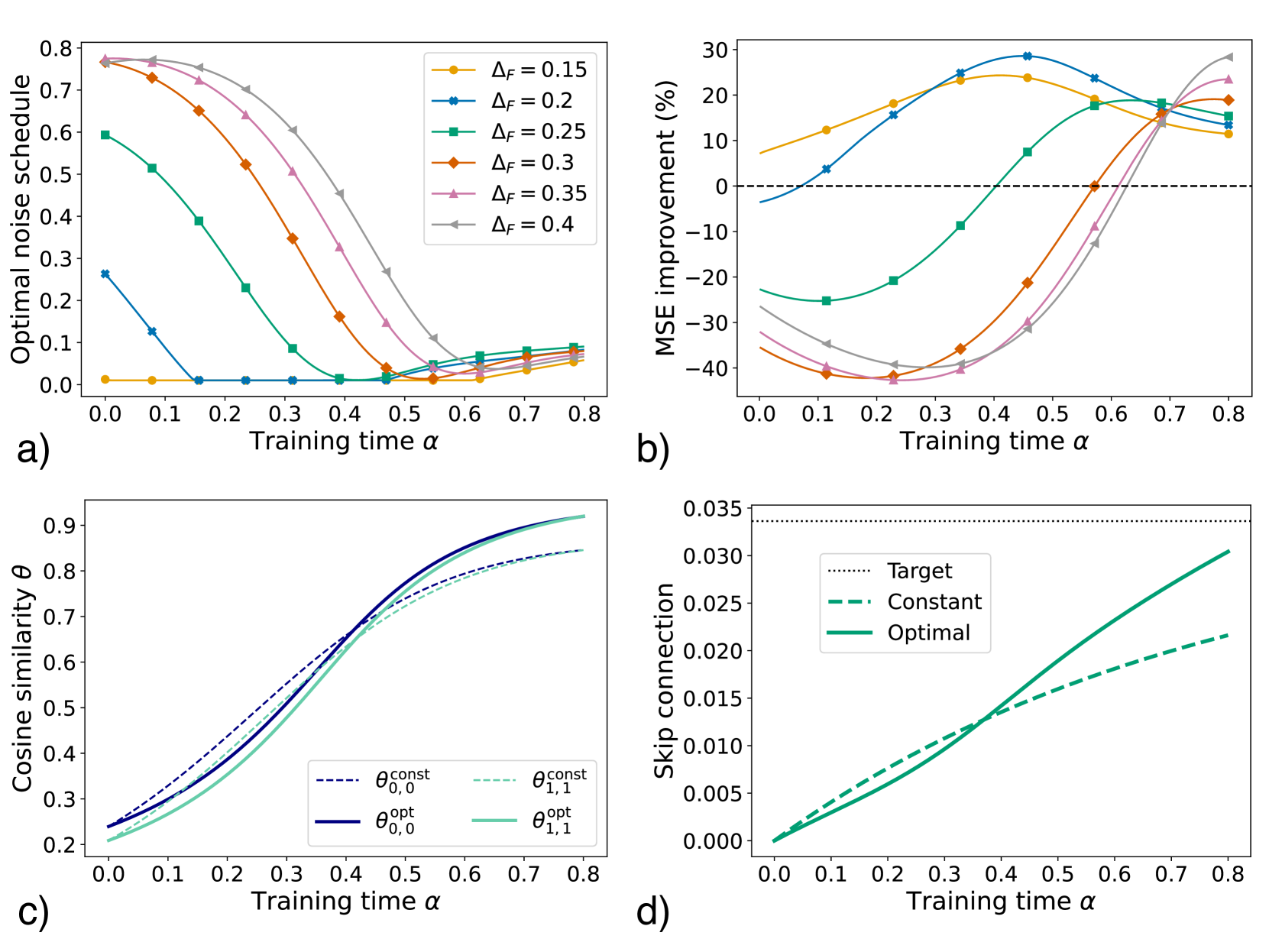
## 2x2 Grid of Subplots: Training Dynamics Analysis ### Overview The image contains four subplots (a-d) analyzing training dynamics across different parameters. Each subplot examines how specific metrics evolve with training time (α) under varying conditions. The visualizations include line graphs with distinct color-coded data series, legends, and axis labels. --- ### Components/Axes #### Subplot a) - **X-axis**: Training time (α) ranging from 0.0 to 0.8 - **Y-axis**: Optimal noise schedule (0.0 to 0.8) - **Legend**: ΔF values (0.15, 0.2, 0.25, 0.3, 0.35, 0.4) with corresponding colors (orange, blue, green, red, pink, gray) - **Line styles**: Solid lines for all series #### Subplot b) - **X-axis**: Training time (α) from 0.0 to 0.8 - **Y-axis**: MSE improvement (%) from -40% to 30% - **Legend**: ΔF values (0.15, 0.2, 0.25, 0.3, 0.35, 0.4) with matching colors - **Line styles**: Solid lines; dashed horizontal line at 0% #### Subplot c) - **X-axis**: Training time (α) from 0.0 to 0.8 - **Y-axis**: Cosine similarity (θ) from 0.2 to 0.9 - **Legend**: - θ_const_0,0 (dashed blue) - θ_const_1,1 (dashed green) - θ_opt_0,0 (solid blue) - θ_opt_1,1 (solid green) #### Subplot d) - **X-axis**: Training time (α) from 0.0 to 0.8 - **Y-axis**: Skip connection (0.000 to 0.035) - **Legend**: - Target (dotted black) - Constant (dashed green) - Optimal (solid green) --- ### Detailed Analysis #### Subplot a) - **Trend**: All ΔF series show decreasing optimal noise schedules as α increases. - **Key values**: - ΔF=0.15 (orange): Starts at ~0.75, ends at ~0.05 - ΔF=0.4 (gray): Starts at ~0.78, ends at ~0.03 - **Spatial grounding**: Legend in top-right; lines originate from top-left and slope downward. #### Subplot b) - **Trend**: MSE improvement varies non-monotonically with α. - **Key values**: - ΔF=0.2 (blue): Peaks at ~25% at α=0.5, then declines to ~10% - ΔF=0.35 (pink): Sharp rise to ~20% at α=0.6, then drops to ~5% - **Spatial grounding**: Legend in top-right; dashed 0% line crosses all series. #### Subplot c) - **Trend**: Cosine similarity improves with α for all θ values. - **Key values**: - θ_opt_0,0 (solid blue): Rises from 0.25 to 0.85 - θ_const_1,1 (dashed green): Increases from 0.22 to 0.75 - **Spatial grounding**: Legend in bottom-left; solid lines outperform dashed. #### Subplot d) - **Trend**: Skip connection increases with α for all series. - **Key values**: - Optimal (solid green): Reaches ~0.035 at α=0.8 - Constant (dashed green): Ends at ~0.025 - **Spatial grounding**: Legend in top-right; solid line dominates. --- ### Key Observations 1. **Noise schedule decay**: Higher ΔF values (e.g., 0.4) achieve lower noise schedules faster (subplot a). 2. **MSE non-linearity**: ΔF=0.2 and 0.35 show peak improvements mid-training (subplot b). 3. **Cosine similarity convergence**: Optimal θ values (θ_opt) outperform constant θ (subplot c). 4. **Skip connection growth**: Optimal skip connections grow fastest (subplot d). --- ### Interpretation The data suggests that: - **Training time α** is critical for optimizing noise schedules (a) and skip connections (d), with diminishing returns at higher α. - **ΔF tuning** impacts MSE improvement non-linearly (b), with mid-range values (0.2–0.35) yielding peak performance. - **θ optimization** (subplot c) demonstrates that adaptive θ values (θ_opt) significantly outperform fixed θ (θ_const), particularly for θ_1,1. - **Skip connection growth** (d) correlates with improved model performance, as higher connections likely enhance gradient flow. These trends highlight the importance of balancing ΔF, θ, and skip connection strategies during training to maximize model efficiency and accuracy.