## Diagram: Jointree, Causal Graph, and Thinned Jointree
### Overview
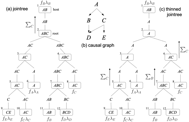
The image presents three diagrams: a jointree, a causal graph, and a thinned jointree. These diagrams illustrate relationships between variables, potentially in the context of probabilistic graphical models or Bayesian networks. The jointree diagrams show a hierarchical structure with nodes labeled with variable sets, while the causal graph depicts direct dependencies between variables. The thinned jointree is a simplified version of the jointree.
### Components/Axes
**(a) Jointree:**
* **Nodes:** Rectangular boxes containing sets of variables (e.g., AB, ABC, AC, A, BC, BCD, CE). Each node is numbered from 1 to 12.
* **Edges:** Lines connecting the nodes, indicating relationships or message passing.
* **Labels:**
* Node 1: "fBλB" (top-left of the node), "host" (top-right of the node)
* Node 2: "root" (right of the node)
* Node 6: "fAλA" (below the node)
* Node 8: "fC" (below the node)
* Node 9: "fEλE" (below the node)
* Node 10: "fCλC" (below the node)
* Node 11: "fB" (below the node)
* Node 12: "fDλD" (below the node)
* **Arrow:** An upward-pointing arrow labeled "ΣC" indicates a summation or marginalization operation.
**(b) Causal Graph:**
* **Nodes:** Labeled A, B, C, D, and E.
* **Edges:** Directed arrows indicating causal relationships. A causes B and C. B causes D. C causes E.
**(c) Thinned Jointree:**
* **Nodes:** Rectangular boxes containing sets of variables (A, AC, AB, BCD, CE). Each node is numbered from 1 to 12.
* **Edges:** Lines connecting the nodes.
* **Labels:**
* Node 1: "fBλB" (top-left of the node)
* Node 6: "fAλA" (below the node)
* Node 8: "fC" (below the node)
* Node 9: "fEλE" (below the node)
* Node 10: "fCλC" (below the node)
* Node 11: "fB" (below the node)
* Node 12: "fDλD" (below the node)
* **Arrows:** Upward-pointing arrows labeled "ΣC" and "ΣB" indicate summation or marginalization operations.
### Detailed Analysis or Content Details
**Jointree (a):**
* Node 1 (AB) is the host.
* Node 2 (ABC) is the root.
* The tree branches from the root (ABC) to nodes 3 (AC) and 4 (ABC).
* Node 3 (AC) branches to nodes 5 (AC) and 6 (A).
* Node 4 (ABC) branches to nodes 7 (ABC) and 8 (AC).
* Node 5 (AC) branches to nodes 9 (CE) and 10 (AC).
* Node 7 (ABC) branches to nodes 11 (AB) and 12 (BCD).
**Causal Graph (b):**
* A is the parent node of B and C.
* B is the parent node of D.
* C is the parent node of E.
**Thinned Jointree (c):**
* Node 1 (AB) is at the top.
* Node 2 (A) is below Node 1.
* The tree branches from Node 2 (A) to nodes 3 (A) and 4 (AC).
* Node 3 (A) branches to nodes 5 (AC) and 6 (A).
* Node 4 (AC) branches to nodes 7 (ABC) and 8 (AC).
* Node 5 (AC) branches to nodes 9 (CE) and 10 (AC).
* Node 7 (ABC) branches to nodes 11 (AB) and 12 (BCD).
### Key Observations
* The jointree and thinned jointree represent factorized probability distributions.
* The causal graph shows the dependencies between variables.
* The thinned jointree is a simplified version of the jointree, potentially optimized for inference.
* The "Σ" symbols indicate marginalization operations, which are used to eliminate variables from the distribution.
### Interpretation
The diagrams illustrate the process of converting a causal model (represented by the causal graph) into a form suitable for efficient inference (represented by the jointree and thinned jointree). The causal graph explicitly shows the dependencies between variables, while the jointree represents the joint probability distribution in a factorized form. The thinned jointree is a further simplification, potentially achieved by eliminating redundant variables or factors. The marginalization operations (ΣC, ΣB) are used to compute marginal probabilities by summing over the possible values of the eliminated variables. The labels "fBλB", "fAλA", etc., likely represent factors in the joint probability distribution. The "host" and "root" labels in the jointree indicate specific roles of nodes in the message-passing process.