\n
## Diagram: Jointree, Causal Graph, and Thinned Jointree
### Overview
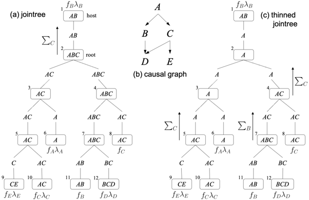
The image presents three diagrams: a jointree (a), a causal graph (b), and a thinned jointree (c). All three diagrams represent relationships between variables A, B, C, D, and E. The diagrams use nodes (rectangles) to represent combinations of variables and arrows to indicate dependencies or conditional probabilities. Each node is labeled with a combination of variables and a number (1-12) indicating a specific step or state in the process. Each arrow is labeled with a function representing a conditional probability.
### Components/Axes
The diagrams share the following components:
* **Nodes:** Rectangular boxes representing combinations of variables (e.g., AB, AC, ABC).
* **Arrows:** Indicate dependencies or conditional probabilities between nodes.
* **Labels on Arrows:** Functions like f<sub>B∧B</sub>, f<sub>A</sub>, f<sub>C</sub>, f<sub>D</sub>, f<sub>E</sub>, etc., representing conditional probabilities.
* **Variables:** A, B, C, D, and E.
* **Σ:** Symbol indicating summation or marginalization.
* **Labels:** "host", "root".
### Detailed Analysis or Content Details
**Diagram (a): Jointree**
* **Node 1:** `AB` labeled "host", with an incoming arrow from `f<sub>B∧B</sub>`.
* **Node 2:** `ABC` labeled "root", with an incoming arrow from `Σ`.
* **Node 3:** `AC`, with an incoming arrow from `ABC`.
* **Node 4:** `ABC`, with an incoming arrow from `AC`.
* **Node 5:** `AC`, with an incoming arrow from `ABC`.
* **Node 6:** `A`, with an incoming arrow from `f<sub>A∧A</sub>`.
* **Node 7:** `ABC`, with an incoming arrow from `AC`.
* **Node 8:** `AC`, with an incoming arrow from `f<sub>C</sub>`.
* **Node 9:** `CE`, with an incoming arrow from `f<sub>E∧E</sub>`.
* **Node 10:** `AC`, with an incoming arrow from `f<sub>C∧C</sub>`.
* **Node 11:** `AB`, with an incoming arrow from `f<sub>B</sub>`.
* **Node 12:** `BCD`, with an incoming arrow from `f<sub>D∧D</sub>`.
* An arrow from `Σ` points to `ABC` (Node 2).
**Diagram (b): Causal Graph**
* **Node A:** At the top, with arrows pointing to B, C, D, and E.
* **Node B:** Receives an arrow from A.
* **Node C:** Receives an arrow from A.
* **Node D:** Receives an arrow from A.
* **Node E:** Receives an arrow from A.
* **Node 5:** `C`, with an incoming arrow from `Σ`.
* **Node 6:** `A`, with an incoming arrow from `f<sub>A∧A</sub>`.
* **Node 7:** `ABC`, with an incoming arrow from `AB`.
* **Node 8:** `AC`, with an incoming arrow from `f<sub>C</sub>`.
* **Node 9:** `CE`, with an incoming arrow from `f<sub>E∧E</sub>`.
* **Node 10:** `AC`, with an incoming arrow from `f<sub>C∧C</sub>`.
* **Node 11:** `AB`, with an incoming arrow from `f<sub>B</sub>`.
* **Node 12:** `BCD`, with an incoming arrow from `f<sub>D∧D</sub>`.
* An arrow from `Σ` points to `C` (Node 5).
**Diagram (c): Thinned Jointree**
* **Node 1:** `AB`, with an incoming arrow from `f<sub>B∧B</sub>`.
* **Node 2:** `A`, with an incoming arrow from `Σ`.
* **Node 3:** `A`, with an incoming arrow from `A`.
* **Node 4:** `AC`, with an incoming arrow from `AC`.
* **Node 5:** `Σ`, points to `A` (Node 2).
* **Node 6:** `A`, with an incoming arrow from `f<sub>A∧A</sub>`.
* **Node 7:** `ABC`, with an incoming arrow from `AC`.
* **Node 8:** `AC`, with an incoming arrow from `f<sub>C</sub>`.
* **Node 9:** `CE`, with an incoming arrow from `f<sub>E∧E</sub>`.
* **Node 10:** `AC`, with an incoming arrow from `f<sub>C∧C</sub>`.
* **Node 11:** `AB`, with an incoming arrow from `f<sub>B</sub>`.
* **Node 12:** `BCD`, with an incoming arrow from `f<sub>D∧D</sub>`.
* An arrow from `Σ` points to `A` (Node 2).
### Key Observations
* All three diagrams represent the same set of variables (A, B, C, D, E).
* The causal graph (b) shows a clear hierarchical structure with A as the root cause influencing B, C, D, and E.
* The jointree (a) and thinned jointree (c) represent the same relationships but with different levels of detail and complexity. The thinned jointree (c) appears to be a simplified version of the jointree (a).
* The functions labeled on the arrows (e.g., f<sub>B∧B</sub>, f<sub>A</sub>) likely represent conditional probabilities.
* The summation symbol (Σ) indicates marginalization or summing over possible values of other variables.
### Interpretation
These diagrams likely illustrate a process of probabilistic inference or belief propagation in a Bayesian network. The causal graph (b) represents the underlying causal relationships between the variables. The jointree (a) is a graphical representation of the factorization of the joint probability distribution over all variables. The thinned jointree (c) is a simplification of the jointree, potentially used for more efficient computation.
The functions on the arrows represent conditional probabilities, and the summation symbol indicates the process of marginalizing out variables to obtain the probability of a particular event. The diagrams demonstrate how to represent and manipulate probabilistic relationships between variables in a graphical model. The progression from causal graph to jointree to thinned jointree suggests a process of model construction and simplification for computational efficiency. The labels "host" and "root" likely refer to specific roles or states within the network. The numbers (1-12) likely represent a sequence of steps in an algorithm or process.