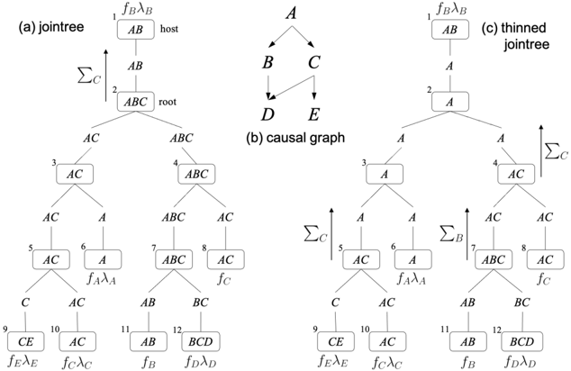
## Diagram Set: Jointree, Causal Graph, and Thinned Jointree ### Overview The image displays three interconnected diagrams illustrating concepts from probabilistic graphical models, specifically Bayesian networks and their junction tree (jointree) representations. The diagrams are labeled (a) jointree, (b) causal graph, and (c) thinned jointree. They are presented side-by-side in a horizontal layout on a white background. All text and lines are in black. ### Components/Axes The image is segmented into three distinct regions: 1. **Left Region (a):** A detailed jointree structure. 2. **Center Region (b):** A simple directed acyclic graph (DAG), the causal graph. 3. **Right Region (c):** A "thinned" version of the jointree from (a). **Common Elements Across Diagrams:** * **Nodes:** Represented by rectangles containing variable sets (e.g., `AB`, `ABC`). * **Edges:** Solid lines connecting nodes, indicating adjacency or separation in the graph. * **Mathematical Annotations:** Functions (e.g., `f_Bλ_B`) and summation symbols (`Σ`) with subscripts (e.g., `Σ_C`) placed near specific nodes. * **Node Numbering:** Small numbers (1-12) in the top-left corner of each node in diagrams (a) and (c). ### Detailed Analysis #### **Diagram (a): Jointree** * **Structure:** A tree-like structure with 12 numbered nodes arranged in a hierarchical, branching layout. * **Node List & Content (Top to Bottom, Left to Right):** * **Node 1 (Top Center):** `AB`. Annotation above: `f_Bλ_B`. Label to the right: `host`. * **Node 2 (Below Node 1):** `ABC`. Label to the right: `root`. An arrow points upward from Node 2 to Node 1, labeled `Σ_C`. * **Node 3 (Left branch from Node 2):** `AC`. * **Node 4 (Right branch from Node 2):** `ABC`. * **Node 5 (Left branch from Node 3):** `AC`. * **Node 6 (Right branch from Node 3):** `A`. Annotation below: `f_Aλ_A`. * **Node 7 (Left branch from Node 4):** `ABC`. * **Node 8 (Right branch from Node 4):** `AC`. Annotation below: `f_C`. * **Node 9 (Left branch from Node 5):** `CE`. Annotation below: `f_Eλ_E`. * **Node 10 (Right branch from Node 5):** `AC`. Annotation below: `f_Cλ_C`. * **Node 11 (Left branch from Node 7):** `AB`. Annotation below: `f_B`. * **Node 12 (Right branch from Node 7):** `BCD`. Annotation below: `f_Dλ_D`. * **Edge Labels:** The edges between nodes are labeled with the separator sets (e.g., `AB`, `AC`, `A`, `C`, `BC`). For example, the edge between Node 2 (`ABC`) and Node 3 (`AC`) is labeled `AC`. #### **Diagram (b): Causal Graph** * **Structure:** A simple directed acyclic graph (DAG) with 5 nodes. * **Node List & Content:** * Top Node: `A` * Middle Left Node: `B` * Middle Right Node: `C` * Bottom Left Node: `D` * Bottom Right Node: `E` * **Edge Directions (Flow):** * `A` → `B` * `A` → `C` * `B` → `D` * `C` → `D` * `C` → `E` #### **Diagram (c): Thinned Jointree** * **Structure:** A modified version of the jointree in (a), also with 12 numbered nodes in the same spatial layout. The key difference is the content of several nodes, which have been simplified or "thinned." * **Node List & Content (Highlighting Changes from (a)):** * **Node 1:** `AB`. Annotation above: `f_Bλ_B`. (Same as (a)) * **Node 2:** `A`. (Changed from `ABC` in (a)). Arrow `Σ_C` points upward to Node 1. * **Node 3:** `A`. (Changed from `AC` in (a)). * **Node 4:** `AC`. (Changed from `ABC` in (a)). Arrow `Σ_C` points upward from Node 4. * **Node 5:** `AC`. (Same as (a)). Arrow `Σ_C` points upward from Node 5. * **Node 6:** `A`. Annotation below: `f_Aλ_A`. (Same as (a)). * **Node 7:** `ABC`. (Same as (a)). Arrow `Σ_B` points upward from Node 7. * **Node 8:** `AC`. Annotation below: `f_C`. (Same as (a)). * **Node 9:** `CE`. Annotation below: `f_Eλ_E`. (Same as (a)). * **Node 10:** `AC`. Annotation below: `f_Cλ_C`. (Same as (a)). * **Node 11:** `AB`. Annotation below: `f_B`. (Same as (a)). * **Node 12:** `BCD`. Annotation below: `f_Dλ_D`. (Same as (a)). * **Edge Labels:** Similar to (a), edges are labeled with separator sets (e.g., `A`, `AC`, `C`, `AB`, `BC`). ### Key Observations 1. **Structural Relationship:** Diagram (b) is the underlying causal model. Diagrams (a) and (c) are two different junction tree representations derived from a graph that includes the variables in (b) plus potentially others (like `F` implied by `f_C`). 2. **Thinning Process:** The transformation from (a) to (c) involves simplifying nodes by removing variables that are not sepset-relevant for message passing in certain parts of the tree. For example, Node 2 changes from `ABC` to `A`, and Node 3 from `AC` to `A`. 3. **Message Passing Annotations:** The `Σ` symbols with subscripts (e.g., `Σ_C`) indicate points in the tree where marginalization (summing out a variable) occurs during belief propagation. Their placement changes between (a) and (c) due to the thinning. 4. **Functional Assignments:** The `f_` and `λ_` terms (e.g., `f_Bλ_B`, `f_Aλ_A`) represent probability distributions or potential functions associated with specific cliques (nodes) in the network. Their placement is consistent between (a) and (c). ### Interpretation This set of diagrams serves as a technical illustration for explaining inference in Bayesian networks. The **causal graph (b)** defines the probabilistic dependencies between variables A, B, C, D, and E. The **jointree (a)** is a data structure constructed to enable exact inference (like computing marginal probabilities) via the junction tree algorithm. Each node is a "clique" of variables, and the tree structure ensures that information (messages) can be passed efficiently between cliques. The **thinned jointree (c)** demonstrates an optimization. By removing variables from cliques where they are not needed for the sepset conditions (the labels on the edges), the computational and storage requirements for inference can be reduced without affecting the final results. The annotations (`Σ_C`, `f_Aλ_A`, etc.) explicitly show where mathematical operations (marginalization) and data (potentials) reside within this algorithmic framework. The progression from (b) to (a) to (c) visually narrates the process of taking a causal model, building a standard inference structure, and then refining it for efficiency.