## Diagram Analysis: Probabilistic Graphical Models
### Overview
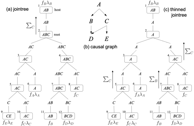
The image presents three interconnected diagrams illustrating probabilistic graphical models: (a) a jointree structure, (b) a causal graph, and (c) a thinned jointree. These diagrams use nodes labeled with variable combinations (e.g., AB, ABC) and directional arrows to represent dependencies, conditional probabilities, and hierarchical relationships.
---
### Components/Axes
#### Diagram (a): Jointree
- **Nodes**:
- Root: `ABC` (labeled "root")
- Intermediate: `AB` (labeled "host"), `AC`, `ABC`
- Leaf: `AC`, `A`, `AB`, `BC`, `CE`, `BCD`
- **Functions**:
- `f_Bλ_B` (node 1), `f_Aλ_A` (node 6), `f_Cλ_C` (node 10), `f_Dλ_D` (node 12)
- **Arrows**:
- Directed edges from parent to child nodes (e.g., `ABC` → `AC`, `AB`).
- **Summation Symbols**:
- `Σ_C` (top-left of diagram).
#### Diagram (b): Causal Graph
- **Nodes**:
- Variables: `A`, `B`, `C`, `D`, `E`
- **Arrows**:
- Bidirectional edges between `B` and `C`, `C` and `D`, `D` and `E`.
- Unidirectional edges from `A` to `B` and `C`.
#### Diagram (c): Thinned Jointree
- **Nodes**:
- Root: `A` (labeled "host")
- Intermediate: `AC`, `ABC`
- Leaf: `AC`, `A`, `AB`, `BC`, `CE`, `BCD`
- **Functions**:
- `f_Bλ_B` (node 1), `f_Aλ_A` (node 6), `f_Cλ_C` (node 10), `f_Dλ_D` (node 12)
- **Arrows**:
- Simplified hierarchy compared to diagram (a), with fewer branching nodes.
- **Summation Symbols**:
- `Σ_C` (top-left) and `Σ_B` (bottom-right).
---
### Detailed Analysis
#### Diagram (a): Jointree
- **Structure**:
- Root node `ABC` branches into `AC` and `AB`.
- `AC` further splits into `AC` (leaf) and `A` (with function `f_Aλ_A`).
- `AB` splits into `ABC` and `AC`, with `ABC` branching into `AB` and `BC`.
- **Functions**:
- Conditional probability terms (e.g., `f_Bλ_B`) are attached to specific nodes, suggesting localized dependencies.
- **Summation**:
- `Σ_C` aggregates contributions from child nodes under `ABC`.
#### Diagram (b): Causal Graph
- **Dependencies**:
- `A` influences `B` and `C` directly.
- `B` and `C` are bidirectionally linked, implying mutual causation.
- `C` influences `D`, which influences `E`, forming a chain of dependencies.
#### Diagram (c): Thinned Jointree
- **Simplification**:
- Reduced branching compared to diagram (a), with `A` as the sole root.
- Nodes like `ABC` and `AC` retain functions from diagram (a), but hierarchical depth is minimized.
- **Functions**:
- Retained terms (`f_Bλ_B`, `f_Aλ_A`) indicate preserved conditional relationships despite simplification.
---
### Key Observations
1. **Hierarchical Reduction**: Diagram (c) simplifies diagram (a) by collapsing intermediate nodes (e.g., `AB` → `A`).
2. **Causal vs. Probabilistic**: Diagram (b) emphasizes bidirectional causation (e.g., `B` ↔ `C`), while diagrams (a) and (c) focus on hierarchical probability distributions.
3. **Function Localization**: Functions like `f_Bλ_B` are consistently placed at nodes representing variable combinations (e.g., `AB`), suggesting localized dependency modeling.
4. **Summation Scope**: `Σ_C` and `Σ_B` in diagrams (a) and (c) indicate aggregation over specific variable subsets.
---
### Interpretation
These diagrams likely represent components of a Bayesian network or factor graph used for probabilistic inference.
- **Diagram (a)** models joint probability distributions over variables (e.g., `ABC`), with functions encoding conditional probabilities.
- **Diagram (b)** highlights causal relationships, where bidirectional edges (e.g., `B` ↔ `C`) suggest confounding or feedback loops.
- **Diagram (c)** demonstrates model simplification, retaining critical dependencies (e.g., `f_Aλ_A`) while reducing computational complexity.
The thinned jointree (c) may serve as an optimized version of the full jointree (a), balancing accuracy and efficiency. The causal graph (b) provides context for how variables interact, which informs the structure of the jointrees. Notably, the absence of numerical values suggests these diagrams are schematic, focusing on structural relationships rather than empirical data.