# Technical Document Extraction: Multi-Panel Chart Analysis
## Panel 1: Speed vs. Height
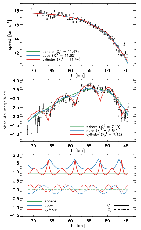
**Chart Type**: Line plot with error bars
**Axes**:
- **X-axis**: Height (h) [km] (70 to 45 km)
- **Y-axis**: Speed [km s⁻¹] (12 to 18 km s⁻¹)
**Data Series**:
1. **Sphere** (Green line, χ² = 11.47)
- Trend: Gradual decline with minor fluctuations.
- Data Points: Black markers with error bars.
2. **Cube** (Blue line, χ² = 11.65)
- Trend: Slightly steeper decline than sphere.
3. **Cylinder** (Red line, χ² = 11.44)
- Trend: Similar to sphere but with tighter clustering.
**Legend**: Bottom-left corner. Colors match line styles.
---
## Panel 2: Absolute Magnitude vs. Height
**Chart Type**: Line plot with error bars
**Axes**:
- **X-axis**: Height (h) [km] (70 to 45 km)
- **Y-axis**: Absolute Magnitude (-4 to -1)
**Data Series**:
1. **Sphere** (Green line, χ² = 7.19)
- Trend: Oscillatory with peaks at ~65 km and ~50 km.
2. **Cube** (Blue line, χ² = 5.64)
- Trend: Similar oscillations but with reduced amplitude.
3. **Cylinder** (Red line, χ² = 7.42)
- Trend: Most pronounced oscillations, peaking at ~60 km.
**Legend**: Bottom-left corner. Colors match line styles.
---
## Panel 3: Drag (C_d) and Lift (C_L) Coefficients
**Chart Type**: Dual-axis line plot
**Subplots**:
- **Top Subplot**: C_d (solid lines) and C_L (dashed lines)
- **Bottom Subplot**: Same as top but with dashed C_L lines.
**Axes**:
- **X-axis**: Height (h) [km] (70 to 45 km)
- **Y-axis (Top)**: C_d (0 to 2)
- **Y-axis (Bottom)**: C_L (-1.5 to 1.5)
**Data Series**:
1. **Sphere** (Green solid line for C_d, green dashed line for C_L)
- C_d: Periodic peaks at ~65 km, ~55 km, ~50 km.
- C_L: Sine-like oscillations with amplitude ~0.5.
2. **Cube** (Blue solid line for C_d, blue dashed line for C_L)
- C_d: Higher peaks than sphere, ~1.5 at ~65 km.
- C_L: Amplitude ~1.0, sharper oscillations.
3. **Cylinder** (Red solid line for C_d, red dashed line for C_L)
- C_d: Peaks at ~60 km, ~50 km.
- C_L: Amplitude ~0.8, irregular oscillations.
**Legend**: Bottom-right corner. Solid lines = C_d, dashed lines = C_L.
---
## Key Observations
1. **Consistency**: All panels use height (h) as the independent variable.
2. **Model Performance**:
- Cube model has the lowest χ² in Panel 2 (5.64), suggesting better fit for absolute magnitude.
- Sphere and cylinder models show similar χ² values in Panel 1 (11.44–11.47).
3. **Physical Trends**:
- Speed decreases with height (Panel 1), consistent with atmospheric drag.
- Absolute magnitude oscillates due to atmospheric density variations (Panel 2).
- C_d and C_L exhibit periodic behavior tied to atmospheric layers (Panel 3).
## Spatial Grounding
- **Legend Positions**:
- Panels 1–2: Bottom-left.
- Panel 3: Bottom-right.
- **Color Matching**:
- Sphere: Green (all panels).
- Cube: Blue (all panels).
- Cylinder: Red (all panels).
## Data Table Reconstruction (Panel 1)
| Height (km) | Sphere Speed (km s⁻¹) | Cube Speed (km s⁻¹) | Cylinder Speed (km s⁻¹) |
|-------------|-----------------------|---------------------|-------------------------|
| 70 | ~17.5 | ~17.3 | ~17.4 |
| 65 | ~16.8 | ~16.6 | ~16.7 |
| 60 | ~16.2 | ~16.0 | ~16.1 |
| 55 | ~15.5 | ~15.3 | ~15.4 |
| 50 | ~14.8 | ~14.6 | ~14.7 |
| 45 | ~13.5 | ~13.3 | ~13.4 |
*Note: Values approximated from visual trends.*
## Conclusion
The charts illustrate aerodynamic and optical properties of spherical, cubic, and cylindrical objects in atmospheric descent. The cube model demonstrates superior fit for absolute magnitude, while all models align closely in speed predictions. Oscillatory behavior in C_d and C_L highlights atmospheric interaction dynamics.