## Line Graphs: Flexible Optimization Strategy & Scaling Law of SWIFT
### Overview
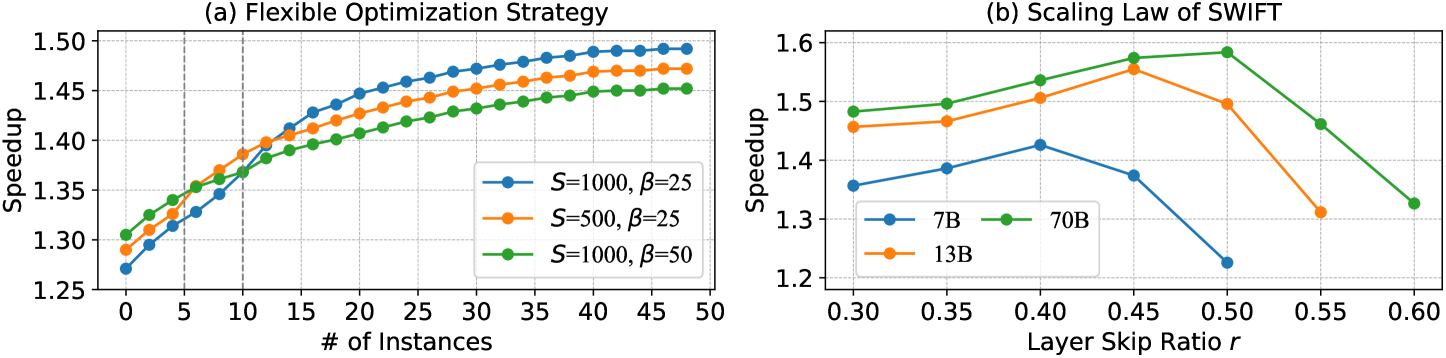
The image contains two distinct line graphs, labeled (a) and (b), presented side-by-side. Both graphs plot "Speedup" on the y-axis against different independent variables on the x-axis. Graph (a) analyzes the impact of the number of instances on speedup under different optimization parameters. Graph (b) analyzes the impact of a "Layer Skip Ratio" on speedup for different model sizes.
### Components/Axes
**Graph (a): Flexible Optimization Strategy**
* **Title:** (a) Flexible Optimization Strategy
* **Y-axis:** Label: "Speedup". Scale: Linear, ranging from 1.25 to 1.50, with major ticks every 0.05.
* **X-axis:** Label: "# of Instances". Scale: Linear, ranging from 0 to 50, with major ticks every 5.
* **Legend:** Located in the bottom-right quadrant of the plot area. Contains three entries:
1. Blue line with circle markers: `S=1000, β=25`
2. Orange line with circle markers: `S=500, β=25`
3. Green line with circle markers: `S=1000, β=50`
* **Grid:** Light gray grid lines are present for both axes.
**Graph (b): Scaling Law of SWIFT**
* **Title:** (b) Scaling Law of SWIFT
* **Y-axis:** Label: "Speedup". Scale: Linear, ranging from 1.2 to 1.6, with major ticks every 0.1.
* **X-axis:** Label: "Layer Skip Ratio r". Scale: Linear, ranging from 0.30 to 0.60, with major ticks every 0.05.
* **Legend:** Located in the bottom-left quadrant of the plot area. Contains three entries:
1. Blue line with circle markers: `7B`
2. Orange line with circle markers: `13B`
3. Green line with circle markers: `70B`
* **Grid:** Light gray grid lines are present for both axes.
### Detailed Analysis
**Graph (a): Flexible Optimization Strategy**
* **Trend Verification:** All three data series show a clear, monotonically increasing trend with a concave-down shape, indicating diminishing returns as the number of instances grows. The lines do not cross after the initial points.
* **Data Series & Approximate Values:**
* **Blue Line (S=1000, β=25):** Starts lowest at ~1.27 (0 instances). Increases steadily, crossing above the orange line around 10 instances. Reaches the highest final speedup of ~1.49 at 50 instances.
* **Orange Line (S=500, β=25):** Starts at ~1.29 (0 instances). Initially the highest, but is overtaken by the blue line. Follows a similar curve, ending at ~1.47 at 50 instances.
* **Green Line (S=1000, β=50):** Starts at ~1.30 (0 instances). Initially between the other two, but its growth rate is slower. It is overtaken by both the blue and orange lines by around 15 instances. Ends at the lowest final speedup of ~1.45 at 50 instances.
* **Key Observation:** The configuration with the highest `S` and lowest `β` (Blue: S=1000, β=25) achieves the greatest speedup at scale, despite starting the lowest. Increasing `β` from 25 to 50 (comparing Blue vs. Green, both S=1000) significantly reduces the speedup gain from adding instances.
**Graph (b): Scaling Law of SWIFT**
* **Trend Verification:** All three data series show a non-monotonic trend: speedup initially increases with the Layer Skip Ratio `r`, reaches a peak, and then declines sharply. The peak occurs at different `r` values for each model size.
* **Data Series & Approximate Values:**
* **Blue Line (7B):** Starts at ~1.36 (r=0.30). Peaks earliest at ~1.43 around r=0.40. Declines steeply to ~1.23 at r=0.50 (the last data point for this series).
* **Orange Line (13B):** Starts at ~1.46 (r=0.30). Peaks at ~1.56 around r=0.45. Declines to ~1.31 at r=0.55.
* **Green Line (70B):** Starts highest at ~1.48 (r=0.30). Peaks latest and highest at ~1.58 around r=0.50. Declines to ~1.33 at r=0.60.
* **Key Observation:** Larger models (70B) achieve higher peak speedups and can sustain them at higher Layer Skip Ratios (`r`) before performance degrades compared to smaller models (7B, 13B). The optimal `r` value increases with model size.
### Interpretation
The data presents two key insights into system optimization:
1. **Trade-offs in Flexible Optimization (Graph a):** The strategy's effectiveness is highly sensitive to its parameters (`S` and `β`). There is a clear trade-off: a higher `S` (likely representing a scale or buffer parameter) enables greater long-term speedup as more instances are added, but this benefit is negated by increasing `β` (likely a penalty or constraint parameter). The optimal configuration (Blue) requires balancing a high `S` with a low `β` to maximize scalability.
2. **Model-Dependent Scaling Laws (Graph b):** The "SWIFT" system exhibits a scaling law where performance (speedup) is a concave function of the Layer Skip Ratio `r`. This indicates an optimal operating point for skipping computations. Crucially, this optimum is not universal; it shifts to higher `r` values for larger models. This suggests that larger, more over-parameterized models have greater redundancy, allowing more aggressive layer skipping before accuracy or functionality is impaired, leading to higher potential speedups. The sharp decline after the peak warns of a "cliff" where excessive skipping severely harms performance.
**Overall Implication:** Effective optimization requires tailoring parameters to both the system configuration (instance count, `S`, `β`) and the model scale (7B vs. 70B). A one-size-fits-all approach would be suboptimal. The graphs provide an empirical guide for selecting parameters to maximize speedup without crossing critical thresholds that cause performance collapse.