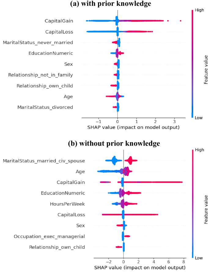
\n ## SHAP Summary Plots: Feature Importance ### Overview The image presents two SHAP (SHapley Additive exPlanations) summary plots, visualizing feature importance in a model. The top plot, labeled "(a) with prior knowledge", shows feature impacts when the model has prior knowledge. The bottom plot, labeled "(b) without prior knowledge", shows feature impacts when the model does not have prior knowledge. Both plots display features on the y-axis and their corresponding SHAP values (impact on model output) on the x-axis. Feature values are indicated by color, ranging from "Low" to "High" on a vertical color bar to the right of each plot. ### Components/Axes Each plot shares the following components: * **X-axis:** "SHAP value (impact on model output)". Scale ranges from approximately -2 to 8 in plot (b) and -1 to 3 in plot (a). * **Y-axis:** Lists of features. * **Color Bar:** Vertical bar on the right indicating "Feature value" from "Low" (blue) to "High" (red). * **Title:** "(a) with prior knowledge" and "(b) without prior knowledge" respectively. Features listed in plot (a): * CapitalGain * CapitalLoss * MaritalStatus_never_married * EducationNumeric * Sex * Relationship_not_in_family * Relationship_own_child * Age * MaritalStatus_divorced Features listed in plot (b): * MaritalStatus_married_civ_spouse * Age * CapitalGain * EducationNumeric * HoursPerWeek * CapitalLoss * Sex * Occupation_exec_managerial * Relationship_own_child ### Detailed Analysis or Content Details **Plot (a) - With Prior Knowledge:** * **CapitalGain:** Shows a wide distribution of SHAP values, centered around 0, with some positive impacts (red dots) and negative impacts (blue dots). The feature values range from low (blue) to high (red). * **CapitalLoss:** Similar to CapitalGain, a wide distribution around 0, with both positive and negative impacts. * **MaritalStatus_never_married:** Primarily negative SHAP values, indicating this feature generally decreases the model output. Feature values are mostly in the mid-range. * **EducationNumeric:** Mostly positive SHAP values, suggesting a positive impact on the model output. Feature values are spread across the range. * **Sex:** Centered around 0, with a slight tendency towards negative SHAP values. * **Relationship_not_in_family:** Predominantly negative SHAP values. * **Relationship_own_child:** Centered around 0, with a slight tendency towards positive SHAP values. * **Age:** Centered around 0, with a slight tendency towards positive SHAP values. * **MaritalStatus_divorced:** Primarily negative SHAP values. **Plot (b) - Without Prior Knowledge:** * **MaritalStatus_married_civ_spouse:** Shows a concentration of positive SHAP values, indicating a strong positive impact on the model output. * **Age:** Shows a wide distribution of SHAP values, centered around 0, with both positive and negative impacts. * **CapitalGain:** Similar to plot (a), a wide distribution around 0, with both positive and negative impacts. * **EducationNumeric:** Mostly positive SHAP values, similar to plot (a). * **HoursPerWeek:** Shows a concentration of negative SHAP values, indicating a negative impact on the model output. * **CapitalLoss:** Similar to plot (a), a wide distribution around 0, with both positive and negative impacts. * **Sex:** Centered around 0, with a slight tendency towards negative SHAP values. * **Occupation_exec_managerial:** Shows a concentration of positive SHAP values. * **Relationship_own_child:** Shows a concentration of negative SHAP values. ### Key Observations * **Feature Importance Shift:** The most important features differ between the two plots. In plot (a), `MaritalStatus_never_married` and `MaritalStatus_divorced` have strong negative impacts. In plot (b), `MaritalStatus_married_civ_spouse` and `Occupation_exec_managerial` have strong positive impacts. * **CapitalGain/CapitalLoss:** These features consistently show a wide distribution of SHAP values in both plots, suggesting their impact is highly variable. * **Age:** The impact of Age is relatively neutral in both plots, with SHAP values centered around 0. * **Color Distribution:** The color distribution within each dot indicates the feature value. For example, red dots in CapitalGain (both plots) represent high CapitalGain values and positive SHAP values, meaning high CapitalGain tends to increase the model output. ### Interpretation These SHAP summary plots demonstrate how feature importance changes when the model is provided with prior knowledge. Plot (a) suggests that, with prior knowledge, marital status (specifically being never married or divorced) has a significant negative impact on the model's output. Plot (b), without prior knowledge, highlights the positive impact of being married and having an executive managerial occupation. The differences in feature importance suggest that prior knowledge acts as a regularizer or constraint, shifting the model's focus to different features. The consistent variability in CapitalGain and CapitalLoss indicates that these features are complex and their impact depends on other factors. The plots provide valuable insights into the model's decision-making process and can be used to identify potential biases or areas for improvement. The color coding allows for a nuanced understanding of how feature values interact with SHAP values to influence the model's predictions. The plots are a visual representation of the model's internal logic, allowing for a more transparent and interpretable machine learning system.