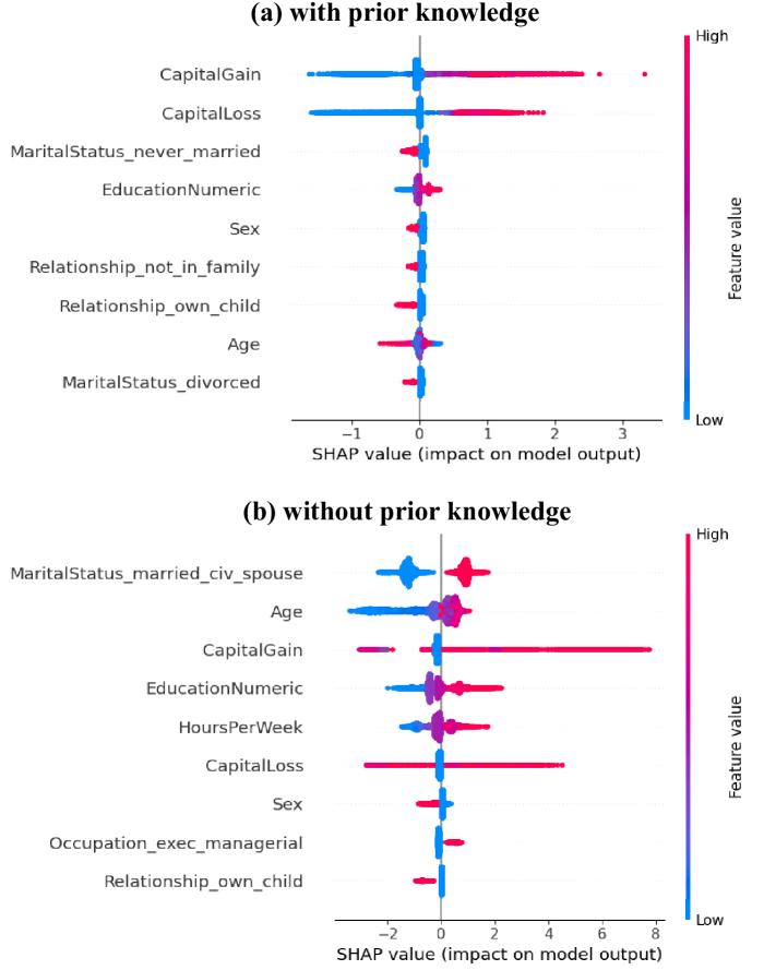
## SHAP Summary Plots: Model Feature Impact Analysis ### Overview The image contains two horizontal SHAP (SHapley Additive exPlanations) summary plots, labeled (a) and (b), which visualize the impact of various features on a machine learning model's output. Plot (a) is titled "with prior knowledge" and plot (b) is titled "without prior knowledge." Each plot displays a set of features on the y-axis and their corresponding SHAP values on the x-axis. The color of each data point represents the feature's value (from low to high), and its position on the x-axis indicates the magnitude and direction of its impact on the model's prediction. ### Components/Axes **Common Elements:** * **Plot Type:** Horizontal SHAP summary (beeswarm) plots. * **X-axis Label:** "SHAP value (impact on model output)" * **Color Legend:** A vertical bar on the right side of each plot labeled "Feature value," with a gradient from **Low (blue)** at the bottom to **High (red)** at the top. * **Feature Labels:** Listed vertically on the left side of each plot. **Plot (a) - "with prior knowledge":** * **X-axis Scale:** Ranges from approximately -1.5 to 3.5. Major tick marks are at -1, 0, 1, 2, 3. * **Features (from top to bottom):** 1. CapitalGain 2. CapitalLoss 3. MaritalStatus_never_married 4. EducationNumeric 5. Sex 6. Relationship_not_in_family 7. Relationship_own_child 8. Age 9. MaritalStatus_divorced **Plot (b) - "without prior knowledge":** * **X-axis Scale:** Ranges from approximately -3 to 8. Major tick marks are at -2, 0, 2, 4, 6, 8. * **Features (from top to bottom):** 1. MaritalStatus_married_civ_spouse 2. Age 3. CapitalGain 4. EducationNumeric 5. HoursPerWeek 6. CapitalLoss 7. Sex 8. Occupation_exec_managerial 9. Relationship_own_child ### Detailed Analysis **Plot (a) - With Prior Knowledge:** * **CapitalGain:** Shows the widest spread. High values (red points) are strongly associated with positive SHAP values (up to ~3.5), indicating they significantly increase the model's output. Low values (blue) cluster around zero or slightly negative impact. * **CapitalLoss:** High values (red) are associated with negative SHAP values (down to ~-1.5), indicating they decrease the model's output. Low values (blue) have a positive impact. * **MaritalStatus_never_married:** High values (red, meaning the status is "never married") have a negative impact (SHAP ~ -0.5). Low values (blue) have a slightly positive impact. * **EducationNumeric:** High values (red) have a moderate positive impact (SHAP ~0.5). Low values (blue) have a slight negative impact. * **Sex:** High values (red, likely representing one gender category) have a small positive impact. Low values (blue) have a small negative impact. * **Relationship_not_in_family:** High values (red) have a negative impact. * **Relationship_own_child:** High values (red) have a negative impact. * **Age:** The distribution is centered near zero, with a slight positive trend for higher values (red). * **MaritalStatus_divorced:** High values (red) have a small negative impact. **Plot (b) - Without Prior Knowledge:** * **MaritalStatus_married_civ_spouse:** High values (red) have a strong positive impact (SHAP ~1.5). Low values (blue) have a strong negative impact (SHAP ~-1.5). * **Age:** High values (red) have a positive impact (SHAP ~1). Low values (blue) have a strong negative impact (SHAP ~-2). * **CapitalGain:** Exhibits the most extreme impact. High values (red) are associated with very large positive SHAP values, extending to nearly 8. Low values (blue) cluster near zero. * **EducationNumeric:** High values (red) have a positive impact (SHAP ~1.5). Low values (blue) have a negative impact. * **HoursPerWeek:** High values (red) have a positive impact. Low values (blue) have a negative impact. * **CapitalLoss:** High values (red) have a strong negative impact (SHAP ~-2). Low values (blue) have a positive impact. * **Sex:** High values (red) have a small positive impact. * **Occupation_exec_managerial:** High values (red) have a positive impact (SHAP ~0.5). * **Relationship_own_child:** High values (red) have a negative impact. ### Key Observations 1. **Scale Difference:** The x-axis scale in plot (b) is more than twice as wide as in plot (a), indicating that feature impacts are generally larger in magnitude when the model operates "without prior knowledge." 2. **Feature Importance Shift:** The top-ranked feature changes from `CapitalGain` in plot (a) to `MaritalStatus_married_civ_spouse` in plot (b). `Age` also moves from near the bottom in (a) to the second position in (b). 3. **CapitalGain Dominance:** In both plots, `CapitalGain` shows a very strong, asymmetric impact where high values drive predictions up significantly. This effect is dramatically amplified in plot (b). 4. **Consistent Directionality:** For features present in both plots (e.g., `CapitalGain`, `CapitalLoss`, `Age`, `EducationNumeric`, `Sex`, `Relationship_own_child`), the *direction* of impact (positive/negative) for high vs. low values is consistent. 5. **New Features:** Plot (b) introduces features not present in the top list of plot (a), such as `MaritalStatus_married_civ_spouse`, `HoursPerWeek`, and `Occupation_exec_managerial`. ### Interpretation These plots likely compare the feature importance and impact for a model predicting a binary outcome (e.g., income >50K) under two different conditions: one where the model incorporates some form of "prior knowledge" (perhaps through pre-training, feature engineering, or a different algorithmic structure) and one where it does not. * **With Prior Knowledge (a):** The model's decisions are influenced by a more balanced set of features, with impacts contained within a narrower range. This suggests the prior knowledge may act as a regularizer, preventing any single feature from having an outsized, potentially overfitted influence. The model appears to weigh `CapitalGain` and `CapitalLoss` as the most critical financial indicators. * **Without Prior Knowledge (b):** The model relies much more heavily on a few key features, especially demographic ones like marital status and age, and shows extreme sensitivity to `CapitalGain`. The larger SHAP values suggest the model is making more decisive, high-magnitude adjustments based on these features. This could indicate a model that is more directly fitting to surface-level correlations in the data, potentially at the cost of robustness or fairness, as sensitive attributes like marital status and age become dominant drivers. **In essence, the "prior knowledge" appears to temper the model's reliance on a few strong, potentially biased signals, leading to a more distributed and constrained decision-making process.** The absence of this knowledge results in a model that amplifies the impact of specific demographic and financial features to a much greater degree.