## Code Snippet: Python Function for Anisotropy Tensor Reconstruction
### Overview
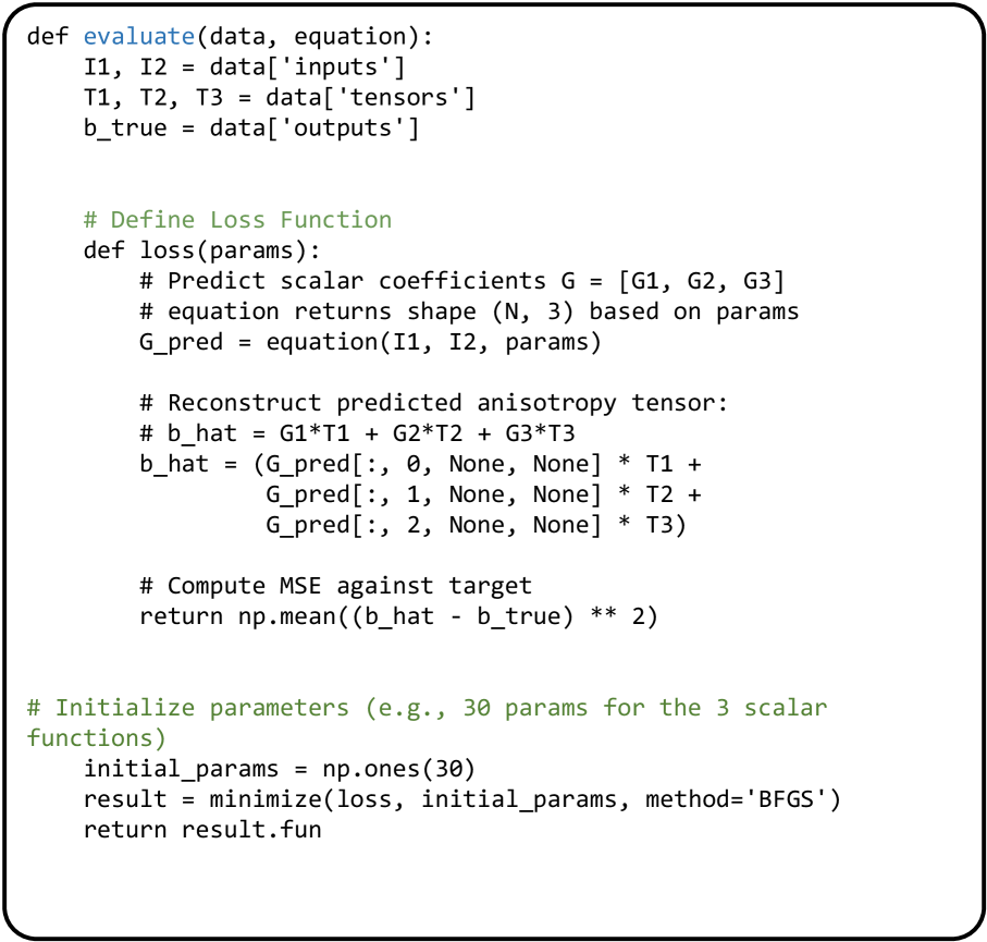
The image displays a Python code snippet defining a function `evaluate` that performs an optimization task. The function's purpose is to train a model (represented by the `equation` callable) to predict scalar coefficients (`G1, G2, G3`) which are then used to reconstruct a target anisotropy tensor (`b_true`). The training minimizes the Mean Squared Error (MSE) between the predicted and true tensors using the BFGS optimization algorithm.
### Components/Axes
The code is structured into two main parts:
1. **Outer Function `evaluate(data, equation)`**: The main entry point that unpacks input data and orchestrates the optimization.
2. **Inner Function `loss(params)`**: Defines the objective function to be minimized. It contains the core logic for prediction, reconstruction, and error calculation.
3. **Optimization Block**: Initializes parameters and runs the minimization routine.
**Key Variables and Functions:**
* `data`: A dictionary containing the dataset with keys `'inputs'`, `'tensors'`, and `'outputs'`.
* `equation`: A callable function that predicts scalar coefficients based on inputs and parameters.
* `I1, I2`: Input variables unpacked from `data['inputs']`.
* `T1, T2, T3`: Component tensors unpacked from `data['tensors']`.
* `b_true`: The target anisotropy tensor from `data['outputs']`.
* `G_pred`: The predicted scalar coefficients, an array of shape `(N, 3)`.
* `b_hat`: The reconstructed anisotropy tensor, calculated as a linear combination: `G1*T1 + G2*T2 + G3*T3`.
* `initial_params`: Initial guess for the model parameters (30 ones).
* `minimize`: The SciPy optimization function used (BFGS method).
* `result.fun`: The final minimized loss value returned by the function.
### Detailed Analysis
The code executes the following logical flow:
1. **Data Unpacking**: The `evaluate` function extracts inputs (`I1, I2`), basis tensors (`T1, T2, T3`), and the ground truth tensor (`b_true`) from the input dictionary.
2. **Loss Function Definition**:
* The inner `loss` function takes model parameters (`params`) as input.
* It calls the provided `equation` function with `I1, I2`, and `params` to generate predictions `G_pred` for the scalar coefficients. The comment notes the expected output shape is `(N, 3)`.
* It reconstructs the predicted anisotropy tensor `b_hat` using broadcasting and element-wise multiplication. The operation is:
`b_hat = (G_pred[:, 0, None, None] * T1) + (G_pred[:, 1, None, None] * T2) + (G_pred[:, 2, None, None] * T3)`
This expands the `(N, 3)` `G_pred` array to match the dimensions of the `T` tensors for the linear combination.
* It computes the Mean Squared Error (MSE) between `b_hat` and `b_true` and returns this scalar loss value.
3. **Optimization Execution**:
* Parameters are initialized as a vector of 30 ones (`initial_params = np.ones(30)`), suggesting the `equation` function has 30 trainable parameters.
* The `minimize` function is called with the `loss` function, initial parameters, and the 'BFGS' method.
* The function returns the final minimized loss value (`result.fun`).
### Key Observations
* **Library Dependencies**: The code implicitly relies on the NumPy (`np`) library for array operations and the SciPy library's `optimize.minimize` function.
* **Tensor Reconstruction**: The reconstruction of `b_hat` uses NumPy broadcasting (`[:, 0, None, None]`) to align the dimensions of the coefficient vector with the basis tensors `T1, T2, T3`.
* **Optimization Method**: The choice of the BFGS (Broyden–Fletcher–Goldfarb–Shanno) algorithm indicates a gradient-based optimization approach suitable for smooth, unconstrained problems.
* **Parameter Count**: The initialization of 30 parameters implies the `equation` model has a specific architecture with 30 degrees of freedom to learn the mapping from inputs `(I1, I2)` to the three scalar coefficients.
### Interpretation
This code snippet represents a **physics-informed or tensor-reconstruction machine learning pipeline**. The core task is to learn a parametric function (`equation`) that can predict the coefficients (`G1, G2, G3`) of a linear combination of predefined basis tensors (`T1, T2, T3`). The goal is for this combination to accurately reproduce a target anisotropy tensor (`b_true`).
The process is framed as an **inverse problem**: given observed data (`b_true`) and a known model structure (linear combination of `T` tensors), find the parameters of the `equation` that best explain the data. The MSE loss quantifies the reconstruction error.
**Potential Applications:**
* **Material Science**: Modeling anisotropic material properties where the overall tensor is a combination of fundamental modes.
* **Continuum Mechanics**: Identifying constitutive model parameters from experimental or simulation data.
* **Reduced-Order Modeling**: Finding a low-dimensional parametric representation (`G` coefficients) of a complex tensor field.
The code is a template for a **data-driven discovery** process, where the `equation` function could be a neural network or another flexible function approximator, and the optimization finds the parameters that make the physical reconstruction (the linear combination) match the observed reality.