## Python Code Snippet: Anisotropy Tensor Optimization Workflow
### Overview
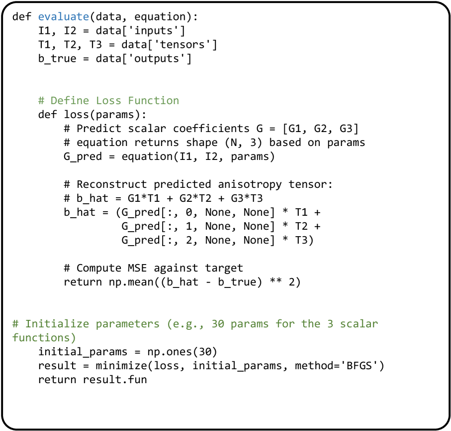
The image contains a Python code snippet implementing an optimization workflow for predicting scalar coefficients of an anisotropy tensor. The code defines functions for evaluation, loss calculation, parameter initialization, and optimization using the BFGS method. Key elements include matrix operations, mean squared error (MSE) computation, and parameter minimization.
### Components/Axes
- **Functions**:
- `evaluate(data, equation)`: Processes input data and applies an equation to generate predictions.
- `loss(params)`: Computes the loss (MSE) between predicted and true anisotropy tensor values.
- **Variables**:
- `I1, I2`: Input data arrays.
- `T1, T2, T3`: Tensor data arrays.
- `b_true`: True output anisotropy tensor.
- `G_pred`: Predicted scalar coefficients (shape `(N, 3)`).
- `b_hat`: Reconstructed anisotropy tensor from predictions.
- **Optimization**:
- `initial_params`: Initialized parameters (30-dimensional array).
- `minimize(loss, initial_params, method='BFGS')`: Optimizes parameters to minimize loss.
### Detailed Analysis
1. **Data Extraction**:
- Inputs (`I1, I2`), tensors (`T1, T2, T3`), and true outputs (`b_true`) are extracted from `data`.
2. **Loss Function**:
- Predicts scalar coefficients `G = [G1, G2, G3]` using `equation(I1, I2, params)`.
- Reconstructs `b_hat` via matrix multiplication: `G_pred[:, 0] * T1 + G_pred[:, 1] * T2 + G_pred[:, 2] * T3`.
- Computes MSE: `np.mean((b_hat - b_true) ** 2)`.
3. **Parameter Initialization**:
- `initial_params = np.ones(30)`: Initializes 30 parameters (likely 10 per scalar function).
- `minimize` uses the BFGS algorithm to find optimal parameters.
### Key Observations
- The code assumes the `equation` function returns a tensor of shape `(N, 3)` based on input parameters.
- The loss function doubles the MSE (`** 2`), which may be a typo or intentional scaling.
- The BFGS method is used for optimization, a quasi-Newton algorithm suitable for smooth, differentiable loss landscapes.
### Interpretation
This code optimizes scalar coefficients (`G1, G2, G3`) to minimize the discrepancy between predicted and true anisotropy tensors. The workflow:
1. **Predicts** coefficients using an equation dependent on inputs and parameters.
2. **Reconstructs** the anisotropy tensor via linear combinations of input tensors.
3. **Optimizes** parameters to reduce MSE, leveraging gradient-based methods (BFGS).
The use of 30 parameters suggests a model with three scalar functions, each requiring 10 parameters (e.g., polynomial coefficients). The doubling of MSE (`** 2`) is ambiguous but could reflect a domain-specific requirement or error in implementation. The BFGS method ensures efficient convergence for smooth loss functions, critical for high-dimensional parameter spaces.