## Line Chart: Percentage of Negative Objects Over Training Epochs
### Overview
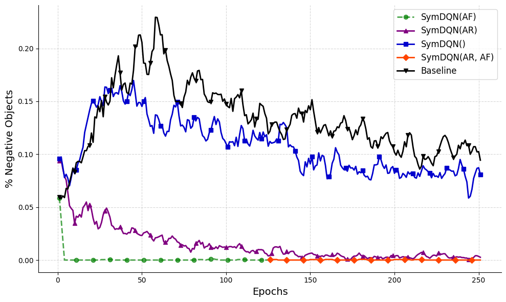
The image displays a line chart comparing the performance of five different reinforcement learning algorithms or variants over the course of 250 training epochs. The performance metric is the percentage of negative objects, where a lower value indicates better performance. The chart shows distinct learning curves and final performance levels for each method.
### Components/Axes
* **X-Axis:** Labeled "Epochs". It represents training time, with major tick marks at 0, 50, 100, 150, 200, and 250.
* **Y-Axis:** Labeled "% Negative Objects". It represents the performance metric, with major tick marks at 0.00, 0.05, 0.10, 0.15, and 0.20.
* **Legend:** Located in the top-right corner of the chart area. It contains five entries, each with a distinct color, line style, and marker:
1. **SymDQN(AF):** Green dashed line with circle markers.
2. **SymDQN(AR):** Purple solid line with triangle-up markers.
3. **SymDQN():** Blue solid line with square markers.
4. **SymDQN(AR, AF):** Orange solid line with diamond markers.
5. **Baseline:** Black solid line with triangle-down markers.
### Detailed Analysis
**Trend Verification & Data Series Analysis:**
1. **SymDQN(AF) (Green, dashed, circles):**
* **Trend:** Starts at approximately 0.06 at epoch 0, then drops precipitously to near 0.00 within the first 10 epochs. It remains flat at or very near 0.00 for the entire remainder of the training (epochs 10-250).
* **Key Points:** Initial value ~0.06 (Epoch 0). Reaches ~0.00 by Epoch ~10. Maintains ~0.00 until Epoch 250.
2. **SymDQN(AR) (Purple, solid, triangles-up):**
* **Trend:** Starts at approximately 0.06 at epoch 0. Shows a rapid initial decrease, followed by a slower, noisy decline. It exhibits significant volatility in the early epochs (0-50) before settling into a gradual downward trend with minor fluctuations.
* **Key Points:** Initial value ~0.06 (Epoch 0). Peaks locally around ~0.055 at Epoch ~15. Declines to ~0.02 by Epoch 50, ~0.01 by Epoch 100, and approaches ~0.00 by Epoch 250, though with slight noise.
3. **SymDQN() (Blue, solid, squares):**
* **Trend:** Starts at approximately 0.095 at epoch 0. Increases sharply to a peak, then enters a long, volatile decline. It shows the second-highest values overall after the Baseline.
* **Key Points:** Initial value ~0.095 (Epoch 0). Rises to a peak of ~0.16 around Epoch 40. Fluctuates between ~0.12 and ~0.15 until Epoch 100. Gradually declines with high volatility, ending at approximately 0.08 at Epoch 250.
4. **SymDQN(AR, AF) (Orange, solid, diamonds):**
* **Trend:** This line is not visible for the first half of the training. It appears at approximately Epoch 125, starting at a value near 0.00. It remains flat at or extremely close to 0.00 from its first appearance until Epoch 250.
* **Key Points:** First visible point at ~Epoch 125, value ~0.00. Maintains ~0.00 until Epoch 250.
5. **Baseline (Black, solid, triangles-down):**
* **Trend:** Starts at approximately 0.06 at epoch 0. Shows the most dramatic increase, reaching the highest peak of all series. After the peak, it enters a volatile, gradual decline but remains the highest-valued series for the entire duration.
* **Key Points:** Initial value ~0.06 (Epoch 0). Rises steeply to a global maximum of ~0.23 around Epoch 60. Fluctuates with a general downward trend, passing through ~0.15 at Epoch 100, ~0.13 at Epoch 150, and ending at approximately 0.10 at Epoch 250.
### Key Observations
* **Performance Hierarchy:** There is a clear and consistent separation in performance. From best (lowest % negative objects) to worst: SymDQN(AF) ≈ SymDQN(AR, AF) > SymDQN(AR) > SymDQN() > Baseline.
* **Convergence:** SymDQN(AF) and SymDQN(AR, AF) converge to near-perfect performance (~0% negative objects) and maintain it. SymDQN(AR) also converges towards zero but with more noise. SymDQN() and the Baseline do not converge to zero within 250 epochs.
* **Volatility:** The Baseline and SymDQN() series exhibit high volatility (large, frequent fluctuations) throughout training. SymDQN(AR) shows moderate volatility early on that decreases over time. SymDQN(AF) and SymDQN(AR, AF) show negligible volatility after convergence.
* **Anomaly:** The SymDQN(AR, AF) series is absent from the plot until approximately epoch 125. This could indicate a delayed start to that specific experiment or a plotting artifact where values were exactly zero and thus not rendered until a change occurred.
### Interpretation
This chart demonstrates the effectiveness of different algorithmic modifications (denoted by AF and AR) to a base SymDQN algorithm in minimizing the production of "negative objects" during training.
* **AF (likely "Action Filtering" or similar) is highly effective:** The SymDQN(AF) variant shows the fastest and most stable convergence to an optimal policy, suggesting this modification is crucial for eliminating negative outcomes.
* **AR (likely "Action Regularization" or similar) is beneficial but slower:** SymDQN(AR) improves significantly over the baseline and base SymDQN(), but its learning is noisier and slower than the AF variant.
* **Combining AR and AF yields perfect final performance:** SymDQN(AR, AF) achieves the same near-zero final performance as SymDQN(AF), though its delayed appearance on the chart is unexplained. It may represent a method that activates or is measured only after a certain training stage.
* **The Baseline algorithm performs poorly:** It not only learns slowly but also actively increases the percentage of negative objects to a high peak before beginning a slow, unstable improvement, highlighting the need for the proposed modifications.
* **Underlying Message:** The data strongly suggests that the proposed SymDQN framework, especially when augmented with the AF mechanism, provides a more stable, efficient, and effective learning process for this task compared to the baseline approach. The clear stratification of the lines provides compelling visual evidence for the superiority of the modified methods.