\n
## State Transition Diagram: Finite Automaton with Interval Constraints
### Overview
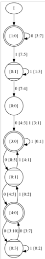
The image displays a vertical state transition diagram, specifically a finite automaton (likely a timed automaton or an automaton with data constraints). It consists of 10 states connected by directed edges (transitions). The states are numbered and some are designated as accepting states (double circles). Transitions are labeled with a format that appears to be `input [min:max]`, suggesting an input symbol and an associated interval constraint, possibly for time or a data value.
### Components/Axes
* **States:** Represented by circles. Each contains a state identifier in square brackets (e.g., `[1:0]`, `[0:1]`).
* **Accepting States:** Indicated by double circles. States `[1:0]`, `[0:1]`, `[3:0]`, and `[4:0]` are accepting states.
* **Start State:** The topmost state, `[1:0]`, is the initial state, indicated by an incoming arrow from a small circle labeled `i`.
* **Transitions:** Directed arrows connecting states. Each has a label in the format `X [a:b]`, where:
* `X` is a single character, likely an input symbol (e.g., `0`, `1`).
* `[a:b]` is an interval, possibly representing a time window, data range, or cost interval.
* **Layout:** The diagram is arranged in a top-down, linear flow with some branching and merging paths.
### Detailed Analysis
**State and Transition Inventory (Top to Bottom):**
1. **Start State `i`** -> Transition `0 [3:7]` -> **State `[1:0]`** (Accepting)
2. **State `[1:0]`**:
* Transition `1 [7:5]` -> **State `[0:1]`** (Accepting)
* Self-loop: `0 [3:7]`
3. **State `[0:1]`**:
* Transition `0 [7:4]` -> **State `[0:0]`**
* Self-loop: `1 [1:3]`
4. **State `[0:0]`**:
* Transition `0 [4:3]` -> **State `[3:0]`** (Accepting)
* Transition `1 [3:1]` -> **State `[3:0]`** (Accepting)
5. **State `[3:0]`** (Accepting):
* Transition `0 [8:5]` -> **State `[4:1]`**
* Transition `1 [0:1]` -> **State `[4:1]`**
6. **State `[4:1]`**:
* Transition `0 [4:5]` -> **State `[4:0]`** (Accepting)
* Transition `1 [0:2]` -> **State `[4:0]`** (Accepting)
7. **State `[4:0]`** (Accepting):
* Transition `0 [3:10]` -> **State `[0:3]`**
* Transition `0 [3:7]` -> **State `[0:3]`** (Note: Two transitions from `[4:0]` to `[0:3]` with input `0` but different intervals).
8. **State `[0:3]`**:
* Transition `1 [0:2]` -> **State `[0:3]`** (Self-loop)
**Key Observations on Structure:**
* The automaton has a clear progression from the start state to the final state `[0:3]`.
* There are multiple paths to reach the accepting state `[3:0]` from `[0:0]`.
* State `[4:0]` has two distinct outgoing transitions for the same input `0`, leading to the same state `[0:3]` but with different interval constraints (`[3:10]` and `[3:7]`). This is a non-deterministic feature.
* The final state `[0:3]` has a self-loop on input `1`.
### Key Observations
1. **Non-determinism:** The transition from state `[4:0]` on input `0` is non-deterministic, as it can choose between two different interval constraints (`[3:10]` or `[3:7]`) to go to the same next state.
2. **Accepting States:** Four of the ten states are accepting states, suggesting multiple points where a processed input string could be considered valid.
3. **Interval Semantics:** The intervals (e.g., `[3:7]`, `[7:5]`) are not consistently ordered (min:max). Some have the first number larger than the second (e.g., `[7:5]`, `[8:5]`). This could indicate they represent a range `[start:end]` where `start > end` is meaningful (e.g., a wrap-around timer, a decreasing counter, or a specific notation for a constraint like `x >= 7 or x <= 5`).
4. **Path Diversity:** There are multiple paths from the start to the final state `[0:3]`, involving different sequences of inputs and interval constraints.
### Interpretation
This diagram represents a **finite state machine with augmented constraints**, most likely a **timed automaton** or an automaton with **data/parameter constraints**.
* **What it models:** It defines a language of sequences (over inputs `0` and `1`) that are accepted if they drive the machine from the start state to any accepting state, while satisfying all the interval constraints encountered along the path. The intervals likely guard the transitions, meaning a transition can only be taken if a certain condition (e.g., a clock value being within the interval `[a:b]`) holds.
* **Purpose:** Such automata are used in formal verification, real-time systems, and protocol analysis to model systems where not just the order of events, but also their timing or associated data values, are critical to correctness.
* **Notable Anomaly:** The intervals where the first number is greater than the second (e.g., `[7:5]`) are particularly interesting. In standard timed automata notation, intervals are usually `min..max` with `min <= max`. This could be a specific notation for this model, perhaps representing a constraint like `x mod 8 ∈ [5,7]` or a different kind of predicate. Without the specific formalism, the exact semantics are ambiguous.
* **Complexity:** The non-determinism in state `[4:0]` and the multiple accepting states indicate a model that can accept a family of related sequences with varying timing/data properties, rather than a single strict sequence. The self-loops (e.g., on `[1:0]`, `[0:1]`, `[0:3]`) allow for loops or waiting periods within the process.
**In essence, this is a specification for a process that consumes inputs `0` and `1`, must adhere to specific numerical constraints at each step, and is considered successful if it ends in one of several designated states.** The diagram is the complete specification of that process's logic.