## Line Chart and Scatter Plot: Magnitude vs. Time and Phase vs. Frequency
### Overview
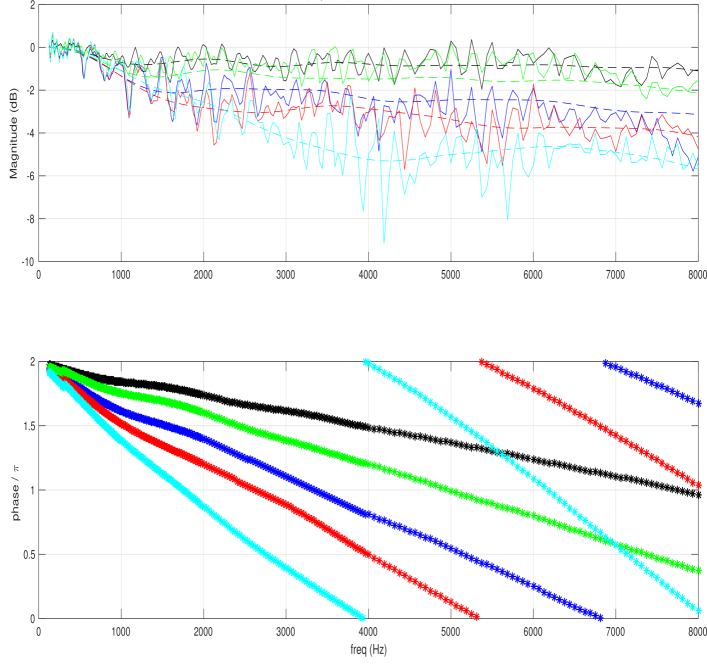
The image contains two subplots:
1. **Top Chart**: A line chart showing multiple colored lines representing magnitude (dB) over time (τ).
2. **Bottom Chart**: A scatter plot with colored dots representing phase (rad) over frequency (Hz), connected by dashed lines.
---
### Components/Axes
#### Top Chart (Line Chart)
- **X-axis**: "τ (time)" with a linear scale from 0 to 8000.
- **Y-axis**: "Magnitude (dB)" with a linear scale from -10 to 2.
- **Legend**: Located on the right, mapping colors to labels:
- Green: "Stable System"
- Purple: "Oscillatory Response"
- Red: "Damped Oscillation"
- Blue: "Low-Frequency Drift"
- Black: "Steep Decay"
- Cyan: "Gradual Decay"
#### Bottom Chart (Scatter Plot)
- **X-axis**: "Frequency (Hz)" with a linear scale from 0 to 8000.
- **Y-axis**: "Phase (rad)" with a linear scale from 0 to 2.
- **Legend**: Implicit via color coding (matches top chart labels).
---
### Detailed Analysis
#### Top Chart Trends
1. **Green Line ("Stable System")**:
- Remains nearly flat around **0 dB** with minor fluctuations (±0.2 dB).
- No significant deviation across the entire time range.
2. **Purple Line ("Oscillatory Response")**:
- Starts at **0 dB**, dips to **-2 dB** at τ ≈ 1000, then oscillates between **-1.5 dB** and **-2.5 dB**.
- Peaks at τ ≈ 3000 (~-1.5 dB) and τ ≈ 7000 (~-2.5 dB).
3. **Red Line ("Damped Oscillation")**:
- Begins at **0 dB**, drops to **-4 dB** at τ ≈ 2000, then fluctuates between **-3.5 dB** and **-4.5 dB**.
- Amplitude decreases slightly over time.
4. **Blue Line ("Low-Frequency Drift")**:
- Starts at **0 dB**, dips to **-6 dB** at τ ≈ 3000, then fluctuates between **-5.5 dB** and **-6.5 dB**.
- Shows a gradual downward trend.
5. **Black Line ("Steep Decay")**:
- Smooth curve from **0 dB** to **-8 dB** at τ ≈ 4000, then plateaus.
6. **Cyan Line ("Gradual Decay")**:
- Smooth curve from **0 dB** to **-10 dB** at τ ≈ 8000, with minimal fluctuations.
#### Bottom Chart Trends
1. **Black Dots (Steep Decay)**:
- Phase decreases from **2 rad** at 1000 Hz to **1 rad** at 8000 Hz.
- Dashed line shows a steep linear decline.
2. **Red Dots (Damped Oscillation)**:
- Phase drops from **2 rad** at 1000 Hz to **0.5 rad** at 6000 Hz.
- Dashed line indicates a moderate decline.
3. **Blue Dots (Low-Frequency Drift)**:
- Phase decreases from **2 rad** at 1000 Hz to **0.2 rad** at 7000 Hz.
- Dashed line shows a gradual decline.
4. **Green Dots (Stable System)**:
- Phase drops from **2 rad** at 1000 Hz to **0.8 rad** at 5000 Hz.
- Dashed line indicates a moderate decline.
5. **Cyan Dots (Gradual Decay)**:
- Phase decreases from **2 rad** at 1000 Hz to **0.4 rad** at 8000 Hz.
- Dashed line shows a steady decline.
---
### Key Observations
1. **Inverse Relationship**:
- Higher magnitude decay (e.g., black/cyan lines) correlates with steeper phase declines (black/cyan dots).
- Stable systems (green line) exhibit minimal phase changes.
2. **Frequency Dependence**:
- All phase trends show decreasing phase with increasing frequency, consistent with typical system dynamics.
3. **Outliers**:
- The blue line ("Low-Frequency Drift") in the top chart has the most pronounced fluctuations, suggesting instability at mid-range frequencies.
---
### Interpretation
- **System Behavior**:
- The top chart illustrates varying stability and response characteristics over time. Systems with steep magnitude decay (black/cyan) exhibit predictable phase declines, while oscillatory systems (purple/red) show erratic behavior.
- The bottom chart confirms that higher-frequency systems (e.g., black/cyan) experience greater phase lag, aligning with classical control theory principles.
- **Design Implications**:
- Systems requiring stability (green line) maintain consistent magnitude and phase, ideal for precision applications.
- Systems with steep decay (black/cyan) may prioritize rapid response but risk phase-related instability at high frequencies.
- **Anomalies**:
- The blue line's mid-range oscillations ("Low-Frequency Drift") suggest potential resonance or unmodeled dynamics, warranting further investigation.
This analysis highlights trade-offs between response speed, stability, and phase coherence in system design.