## Dual-Axis Combination Chart: Gradient Size and Variance over Epochs
### Overview
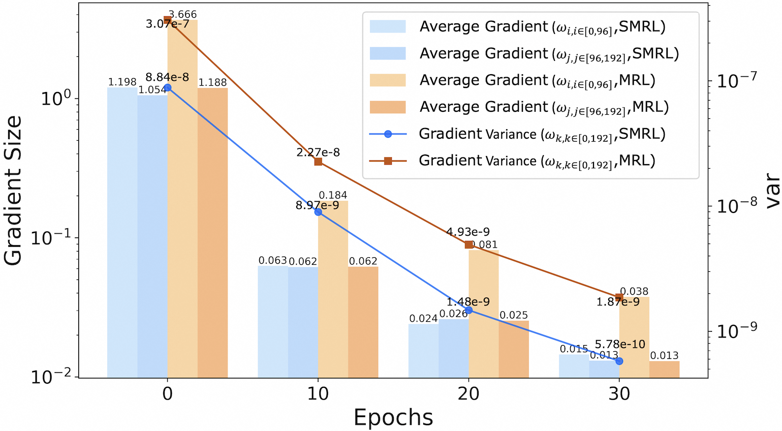
This image is a technical chart combining bar and line plots on a dual y-axis. It visualizes the evolution of gradient statistics (average size and variance) for two different methods, labeled "SMRL" and "MRL," across training epochs. The chart uses a logarithmic scale for both y-axes.
### Components/Axes
* **Chart Type:** Combination bar and line chart with dual y-axes.
* **X-Axis:**
* **Label:** "Epochs"
* **Markers/Ticks:** 0, 10, 20, 30.
* **Primary Y-Axis (Left):**
* **Label:** "Gradient Size"
* **Scale:** Logarithmic (base 10), ranging from 10⁻² to 10⁰.
* **Secondary Y-Axis (Right):**
* **Label:** "var" (presumably variance)
* **Scale:** Logarithmic (base 10), ranging from 10⁻⁹ to 10⁻⁷.
* **Legend (Top-Right Corner):** Contains six entries, differentiating data series by color and marker type.
1. **Light Blue Bar:** `Average Gradient (ω_i,i∈[0,96], SMRL)`
2. **Medium Blue Bar:** `Average Gradient (ω_j,j∈[96,192], SMRL)`
3. **Light Orange Bar:** `Average Gradient (ω_i,i∈[0,96], MRL)`
4. **Dark Orange Bar:** `Average Gradient (ω_j,j∈[96,192], MRL)`
5. **Blue Line with Circle Marker:** `Gradient Variance (ω_k,k∈[0,192], SMRL)`
6. **Brown Line with Square Marker:** `Gradient Variance (ω_k,k∈[0,192], MRL)`
### Detailed Analysis
The chart presents data at four discrete epochs (0, 10, 20, 30). At each epoch, four bars are clustered, and two line data points are plotted.
**Data Series & Trends:**
* **Trend Verification:** All four bar series (average gradients) show a clear, steep downward trend from epoch 0 to 30. Both line series (variances) also show a consistent downward trend.
* **Component Isolation - Epoch 0:**
* **Bars (Gradient Size):**
* SMRL (ω_i,i∈[0,96]): ~1.198
* SMRL (ω_j,j∈[96,192]): ~1.054
* MRL (ω_i,i∈[0,96]): ~3.666 **(Highest initial value)**
* MRL (ω_j,j∈[96,192]): ~1.188
* **Lines (Variance):**
* SMRL Variance: ~8.84e-8
* MRL Variance: ~3.07e-7 **(Highest initial variance)**
* **Component Isolation - Epoch 10:**
* **Bars (Gradient Size):**
* SMRL (ω_i,i∈[0,96]): ~0.063
* SMRL (ω_j,j∈[96,192]): ~0.062
* MRL (ω_i,i∈[0,96]): ~0.184
* MRL (ω_j,j∈[96,192]): ~0.062
* **Lines (Variance):**
* SMRL Variance: ~8.97e-9
* MRL Variance: ~2.27e-8
* **Component Isolation - Epoch 20:**
* **Bars (Gradient Size):**
* SMRL (ω_i,i∈[0,96]): ~0.024
* SMRL (ω_j,j∈[96,192]): ~0.026
* MRL (ω_i,i∈[0,96]): ~0.081
* MRL (ω_j,j∈[96,192]): ~0.025
* **Lines (Variance):**
* SMRL Variance: ~1.48e-9
* MRL Variance: ~4.93e-9
* **Component Isolation - Epoch 30:**
* **Bars (Gradient Size):**
* SMRL (ω_i,i∈[0,96]): ~0.015
* SMRL (ω_j,j∈[96,192]): ~0.013
* MRL (ω_i,i∈[0,96]): ~0.038
* MRL (ω_j,j∈[96,192]): ~0.013
* **Lines (Variance):**
* SMRL Variance: ~5.78e-10
* MRL Variance: ~1.87e-9
### Key Observations
1. **Consistent Decline:** All measured quantities (average gradient sizes for both weight subsets and both methods, as well as overall gradient variance) decrease by approximately two orders of magnitude over 30 epochs.
2. **Method Comparison (MRL vs. SMRL):**
* **Gradient Size:** The MRL method's average gradient for the first weight subset (`ω_i,i∈[0,96]`) starts significantly higher (3.666 vs. 1.198) and remains higher than its SMRL counterpart at every epoch, though the gap narrows.
* **Variance:** The MRL method consistently exhibits higher gradient variance than SMRL at every measured epoch. The initial variance for MRL is about 3.5 times that of SMRL.
3. **Within-Method Comparison:** For both methods, the average gradient sizes for the two different weight subsets (`ω_i` and `ω_j`) become very similar after the initial epoch, suggesting convergence in gradient magnitude across different parts of the model.
4. **Outlier:** The initial average gradient for MRL on `ω_i,i∈[0,96]` (3.666) is a clear outlier, being the largest value on the chart by a significant margin.
### Interpretation
This chart likely analyzes the training dynamics of two machine learning optimization or regularization methods, SMRL and MRL. The data demonstrates that both methods successfully drive down gradient magnitudes and variances over time, which is a typical sign of training convergence and stabilization.
The key investigative insight is the **performance gap between MRL and SMRL**. The consistently higher gradient variance for MRL suggests its optimization landscape may be noisier or less stable than SMRL's. The notably larger initial gradients for MRL could indicate a different parameter initialization scheme, a more aggressive early learning rate, or a fundamental difference in how the method scales gradients. The fact that MRL's gradients start larger but still converge to small values implies the method is effective, but potentially through a different, higher-variance trajectory compared to SMRL. The convergence of gradient sizes between different weight subsets (`ω_i` and `ω_j`) within each method suggests that, over time, the optimization pressure becomes evenly distributed across the model's parameters for both techniques.