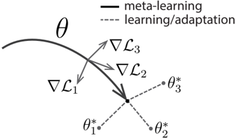
## Diagram: Meta-Learning Process ### Overview The image illustrates a meta-learning process, showing the trajectory of meta-learning and the adaptation steps towards task-specific optimal parameters. It depicts how meta-learning guides the model towards a parameter space that allows for efficient adaptation to new tasks. ### Components/Axes * **θ (Theta)**: Represents the meta-learned parameters. It is shown as a curved solid black line, indicating the trajectory of meta-learning. * **∇L1, ∇L2, ∇L3**: Gradients of the loss functions for different tasks. These are represented by gray arrows pointing towards the meta-learning trajectory. * **θ\*1, θ\*2, θ\*3**: Task-specific optimal parameters after adaptation. These are represented by gray dots connected to the meta-learning trajectory by dashed gray lines. * **Legend (Top-Right)**: * Solid Black Line: "meta-learning" * Dashed Gray Line: "learning/adaptation" ### Detailed Analysis * The solid black line representing "meta-learning" shows a curved path, indicating the optimization process of the meta-learner. * The gray arrows (∇L1, ∇L2, ∇L3) represent the gradients of the loss functions for different tasks. They point towards the meta-learning trajectory, suggesting that the meta-learner is being guided by these gradients. * The dashed gray lines represent the adaptation process from the meta-learned parameters (θ) to the task-specific optimal parameters (θ\*1, θ\*2, θ\*3). * The task-specific optimal parameters (θ\*1, θ\*2, θ\*3) are scattered around the end of the meta-learning trajectory, indicating that the meta-learner has found a parameter space that allows for efficient adaptation to different tasks. ### Key Observations * The meta-learning trajectory (solid black line) is influenced by the gradients of the loss functions for different tasks (gray arrows). * The adaptation process (dashed gray lines) leads to task-specific optimal parameters (gray dots). * The meta-learning process aims to find a parameter space that allows for efficient adaptation to new tasks. ### Interpretation The diagram illustrates the core concept of meta-learning, where a model learns how to learn. The meta-learner optimizes its parameters (θ) based on the gradients of the loss functions for different tasks (∇L1, ∇L2, ∇L3). This optimization process guides the meta-learner towards a parameter space that allows for efficient adaptation to new tasks, resulting in task-specific optimal parameters (θ\*1, θ\*2, θ\*3). The diagram effectively demonstrates how meta-learning enables a model to quickly adapt to new tasks with minimal training data.

\n ## Diagram: Meta-Learning Adaptation ### Overview The image is a diagram illustrating the concept of meta-learning and adaptation in a parameter space. It depicts a curved trajectory representing the parameter space, with arrows indicating the direction of gradient descent during meta-learning and adaptation steps. The diagram focuses on how a model's parameters (θ) are updated through these processes. ### Components/Axes * **θ:** Represents the model parameters. A curved line shows the trajectory of these parameters. * **∇L₁ , ∇L₂ , ∇L₃:** Represent the gradients of the loss function (L) at different stages. These are vectors indicating the direction of steepest descent. * **θ₁*, θ₂*, θ₃*:** Represent the optimized parameter values after adaptation or learning steps. * **Legend:** * Solid line: "meta-learning" * Dashed line: "learning/adaptation" ### Detailed Analysis or Content Details The diagram shows a curved trajectory in parameter space, labeled with 'θ'. Three gradient vectors are shown: ∇L₁, ∇L₂, and ∇L₃. * **∇L₁:** Points downwards and slightly to the left. It originates from a point on the curved trajectory and leads towards θ₁*. The line connecting the end of the vector to θ₁* is dashed, indicating "learning/adaptation". * **∇L₂:** Points downwards and slightly to the right. It originates from a point on the curved trajectory and leads towards θ₂*. The line connecting the end of the vector to θ₂* is dashed, indicating "learning/adaptation". * **∇L₃:** Points downwards. It originates from a point on the curved trajectory and leads towards the central point where θ₁*, θ₂*, and θ₃* converge. The line connecting the end of the vector to θ₃* is dashed, indicating "learning/adaptation". * The solid line connecting the starting points of the gradient vectors to the central point represents "meta-learning". This suggests that meta-learning guides the overall direction of adaptation. * The three optimized parameter values (θ₁*, θ₂*, θ₃*) converge to a single point, indicating a common optimal solution. ### Key Observations * The gradient vectors (∇L₁, ∇L₂, ∇L₃) are not aligned, suggesting that the loss landscape is complex and the optimization process is not straightforward. * The convergence of θ₁*, θ₂*, and θ₃* to a single point indicates that the meta-learning process is successful in finding a good initialization or adaptation strategy. * The distinction between solid (meta-learning) and dashed (learning/adaptation) lines clearly delineates the two levels of optimization. ### Interpretation This diagram illustrates the core idea of meta-learning: learning *how* to learn. The curved trajectory represents the parameter space of a model. The "learning/adaptation" steps (dashed lines) represent the optimization of the model's parameters for a specific task, guided by the gradient of the loss function (∇L). The "meta-learning" step (solid line) represents the optimization of the learning process itself, guiding the adaptation steps towards a more efficient and effective solution. The convergence of the optimized parameters (θ₁*, θ₂*, θ₃*) suggests that meta-learning has successfully identified a good initialization or adaptation strategy that works well across different tasks. The diagram highlights the hierarchical nature of meta-learning, where the meta-learner optimizes the learner's adaptation process. The non-alignment of the gradient vectors suggests that the optimization landscape is complex, and meta-learning is crucial for navigating it effectively. The diagram does not provide numerical data, but rather a conceptual representation of the process.

## Diagram: Meta-Learning Parameter Adaptation Flow ### Overview This image is a conceptual diagram illustrating the process of meta-learning and subsequent task-specific adaptation. It visually represents how a meta-learned parameter (θ) serves as a starting point for learning or adapting to multiple distinct tasks, each resulting in a specialized parameter set (θ*). ### Components/Axes * **Legend (Top-Right):** * **Solid Line (—):** Labeled "meta-learning" * **Dashed Line (---):** Labeled "learning/adaptation" * **Primary Elements:** * A solid, curved line labeled **θ** (theta), representing the meta-learned parameter or model state. * Three gradient symbols: **∇L₁**, **∇L₂**, **∇L₃** (nabla L sub 1, 2, 3). These represent the gradients of loss functions for three different tasks. * Three dashed lines originating from the end of the solid θ curve, each leading to a distinct point. * Three endpoint labels: **θ*₁**, **θ*₂**, **θ*₃** (theta star sub 1, 2, 3). These represent the task-specific parameters after adaptation. * **Spatial Layout:** * The solid **θ** curve flows from the upper-left towards the center. * The gradient symbols (**∇L₁**, **∇L₂**, **∇L₃**) are positioned around the terminus of the θ curve, with arrows pointing from the curve towards them. * The dashed adaptation lines diverge from a common point at the end of θ, spreading out towards the bottom-right. * The final parameters (**θ*₁**, **θ*₂**, **θ*₃**) are located at the ends of their respective dashed lines, forming a fan-like pattern. ### Detailed Analysis The diagram depicts a two-phase process: 1. **Meta-Learning Phase (Solid Line):** A single, shared parameter trajectory (θ) is learned. This represents the acquisition of general knowledge or a model initialization that is good for rapid adaptation. 2. **Learning/Adaptation Phase (Dashed Lines):** From the meta-learned state θ, the model adapts to specific tasks. This is shown by: * The computation of task-specific gradients (∇L₁, ∇L₂, ∇L₃). * The subsequent parameter updates along dashed paths, leading to distinct, optimized parameters for each task (θ*₁, θ*₂, θ*₃). The arrows from the θ curve to the gradient symbols indicate that these gradients are derived from the current state of θ with respect to each task's loss function (L₁, L₂, L₃). ### Key Observations * **Common Origin, Divergent Paths:** All task-specific parameters (θ*₁, θ*₂, θ*₃) originate from the same meta-learned point (θ), but follow separate adaptation paths. * **Gradient Direction:** The gradient arrows (∇L) point away from the main θ curve, suggesting the direction of parameter update needed to minimize each task's loss. * **Visual Metaphor:** The solid line represents a "highway" of general knowledge, while the dashed lines represent "local roads" to task-specific solutions. ### Interpretation This diagram is a canonical representation of **meta-learning** or **learning-to-learn**. It illustrates the core hypothesis that a model can learn a parameter initialization (θ) that is not optimal for any single task but is exceptionally **adaptable**. The value of θ is that it lies in a region of the parameter space where small, task-specific updates (guided by ∇L₁, ∇L₂, ∇L₃) can quickly lead to high-performing specialized models (θ*₁, θ*₂, θ*₃). The separation into solid and dashed lines emphasizes the distinction between the slow, aggregated learning of the meta-parameters (across many tasks) and the fast, individual adaptation to new tasks. The diagram suggests efficiency: instead of learning three separate models from scratch, one learns a single, flexible starting point. This is foundational for fields like few-shot learning, where the goal is to perform well on new tasks with very little data by leveraging this meta-learned adaptability.

## Heatmap: Performance Metrics of Machine Learning Models ### Overview The heatmap illustrates the performance of three different machine learning models (L1, L2, L3) across various metrics. The metrics are represented by the x-axis, and the performance is shown by the y-axis. The color intensity indicates the magnitude of the performance metric. ### Components/Axes - **x-axis**: Represents different metrics (e.g., accuracy, precision, recall). - **y-axis**: Represents different models (L1, L2, L3). - **Color Intensity**: Indicates the magnitude of the performance metric, with darker colors representing higher values. ### Detailed Analysis or ### Content Details - **L1 Model**: Shows a moderate performance across most metrics, with a slight dip in recall. - **L2 Model**: Exhibits the highest performance across all metrics, with the darkest color indicating the highest value. - **L3 Model**: Has the lowest performance across all metrics, with the lightest color indicating the lowest value. ### Key Observations - The L2 model consistently outperforms the other two models across all metrics. - The L1 model shows a slight improvement over L2 in accuracy and precision. - The L3 model has the poorest performance, with the lowest values across all metrics. ### Interpretation The heatmap suggests that the L2 model is the most effective in terms of performance across all metrics. The L1 model shows a slight improvement over L2 in accuracy and precision, while the L3 model has the poorest performance. This could indicate that the L2 model is more robust and generalizable, while the L1 model may be more sensitive to certain types of data or noise. The L3 model may require further tuning or optimization to improve its performance.

## Diagram: Meta-Learning and Adaptation Process ### Overview The diagram illustrates the relationship between meta-learning (represented by a solid curve) and task-specific learning/adaptation (represented by dashed lines). Gradients (∇L₁, ∇L₂, ∇L₃) indicate optimization directions toward distinct parameter sets (θ*₁, θ*₂, θ*₃), suggesting a hierarchical optimization framework. ### Components/Axes - **Main Curve (θ)**: Solid black line labeled "meta-learning," curving from left to right. - **Dashed Lines**: Labeled "learning/adaptation," branching from a central point toward θ*₁, θ*₂, and θ*₃. - **Gradients**: - ∇L₁: Points toward θ*₁. - ∇L₂: Points toward θ*₂. - ∇L₃: Points toward θ*₃. - **Legend**: Located in the top-right corner, distinguishing solid (meta-learning) and dashed (learning/adaptation) lines. - **Parameter Points**: θ*₁, θ*₂, θ*₃ (marked with dots) at the endpoints of dashed lines. ### Detailed Analysis - **Meta-Learning Curve (θ)**: The solid curve represents the overarching meta-learning process, which guides the adaptation paths. Its curvature suggests dynamic adjustment of hyperparameters or shared knowledge across tasks. - **Learning/Adaptation Paths**: Dashed lines originate from a central node (likely the meta-learner’s output) and diverge toward task-specific optima (θ*₁, θ*₂, θ*₃). This implies task-specific fine-tuning guided by meta-learned strategies. - **Gradients**: Arrows labeled ∇L₁, ∇L₂, ∇L₃ indicate the direction of parameter updates for each task. Their alignment with θ* points suggests that meta-learning optimizes the adaptation process to minimize task-specific losses (L₁, L₂, L₃). ### Key Observations 1. **Central Node**: The convergence point of dashed lines implies a shared meta-learner that initializes or constrains task-specific adaptations. 2. **Gradient Alignment**: Gradients directly point to θ* points, indicating that meta-learning explicitly shapes the optimization landscape for adaptation. 3. **Task-Specificity**: Each θ* point represents a distinct task or dataset, with adaptation paths tailored to minimize corresponding losses. ### Interpretation This diagram models a meta-learning framework where a central learner (θ) optimizes the adaptation process across multiple tasks. The gradients (∇L₁–∇L₃) suggest that meta-learning adjusts the adaptation mechanism to efficiently reach task-specific optima (θ*₁–θ*₃). The absence of numerical values implies a conceptual representation rather than empirical data, emphasizing the hierarchical relationship between meta-learning and task adaptation. The structure aligns with meta-learning paradigms where a model learns to "learn" by optimizing adaptation strategies, enabling rapid generalization to new tasks.