\n
## Diagram: Meta-Learning Adaptation
### Overview
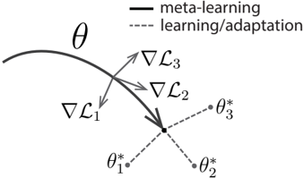
The image is a diagram illustrating the concept of meta-learning and adaptation in a parameter space. It depicts a curved trajectory representing the parameter space, with arrows indicating the direction of gradient descent during meta-learning and adaptation steps. The diagram focuses on how a model's parameters (θ) are updated through these processes.
### Components/Axes
* **θ:** Represents the model parameters. A curved line shows the trajectory of these parameters.
* **∇L₁ , ∇L₂ , ∇L₃:** Represent the gradients of the loss function (L) at different stages. These are vectors indicating the direction of steepest descent.
* **θ₁*, θ₂*, θ₃*:** Represent the optimized parameter values after adaptation or learning steps.
* **Legend:**
* Solid line: "meta-learning"
* Dashed line: "learning/adaptation"
### Detailed Analysis or Content Details
The diagram shows a curved trajectory in parameter space, labeled with 'θ'. Three gradient vectors are shown: ∇L₁, ∇L₂, and ∇L₃.
* **∇L₁:** Points downwards and slightly to the left. It originates from a point on the curved trajectory and leads towards θ₁*. The line connecting the end of the vector to θ₁* is dashed, indicating "learning/adaptation".
* **∇L₂:** Points downwards and slightly to the right. It originates from a point on the curved trajectory and leads towards θ₂*. The line connecting the end of the vector to θ₂* is dashed, indicating "learning/adaptation".
* **∇L₃:** Points downwards. It originates from a point on the curved trajectory and leads towards the central point where θ₁*, θ₂*, and θ₃* converge. The line connecting the end of the vector to θ₃* is dashed, indicating "learning/adaptation".
* The solid line connecting the starting points of the gradient vectors to the central point represents "meta-learning". This suggests that meta-learning guides the overall direction of adaptation.
* The three optimized parameter values (θ₁*, θ₂*, θ₃*) converge to a single point, indicating a common optimal solution.
### Key Observations
* The gradient vectors (∇L₁, ∇L₂, ∇L₃) are not aligned, suggesting that the loss landscape is complex and the optimization process is not straightforward.
* The convergence of θ₁*, θ₂*, and θ₃* to a single point indicates that the meta-learning process is successful in finding a good initialization or adaptation strategy.
* The distinction between solid (meta-learning) and dashed (learning/adaptation) lines clearly delineates the two levels of optimization.
### Interpretation
This diagram illustrates the core idea of meta-learning: learning *how* to learn. The curved trajectory represents the parameter space of a model. The "learning/adaptation" steps (dashed lines) represent the optimization of the model's parameters for a specific task, guided by the gradient of the loss function (∇L). The "meta-learning" step (solid line) represents the optimization of the learning process itself, guiding the adaptation steps towards a more efficient and effective solution.
The convergence of the optimized parameters (θ₁*, θ₂*, θ₃*) suggests that meta-learning has successfully identified a good initialization or adaptation strategy that works well across different tasks. The diagram highlights the hierarchical nature of meta-learning, where the meta-learner optimizes the learner's adaptation process. The non-alignment of the gradient vectors suggests that the optimization landscape is complex, and meta-learning is crucial for navigating it effectively. The diagram does not provide numerical data, but rather a conceptual representation of the process.