## Diagram: Matrix Multiplication and Element-wise Addition
### Overview
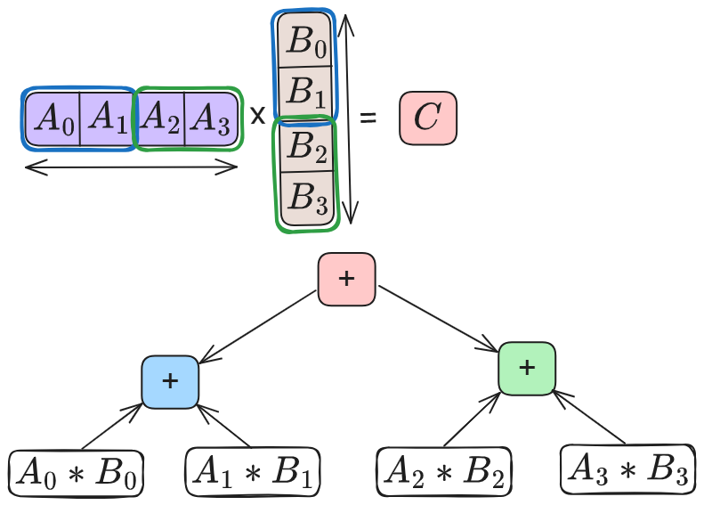
The image depicts a mathematical operation involving two matrices, **A** (1×4) and **B** (4×1), with their product resulting in a scalar value **C**. Below the multiplication, the computation is broken down into intermediate steps: element-wise products of **A** and **B** are summed in pairs, with the final result being the sum of these pairs.
### Components/Axes
- **Matrices**:
- **A**: A 1×4 row matrix labeled `A₀`, `A₁`, `A₂`, `A₃` (purple background).
- **B**: A 4×1 column matrix labeled `B₀`, `B₁`, `B₂`, `B₃` (beige background).
- **Operations**:
- **Multiplication**: Denoted by `×` between matrices **A** and **B**, yielding matrix **C** (pink background).
- **Addition**: Two intermediate sums:
- `A₀*B₀ + A₁*B₁` (blue square).
- `A₂*B₂ + A₃*B₃` (green square).
- **Final Sum**: A pink square labeled `+` connects the two intermediate sums to produce **C**.
### Detailed Analysis
- **Matrix Dimensions**:
- **A**: 1 row × 4 columns.
- **B**: 4 rows × 1 column.
- **C**: 1 row × 1 column (scalar).
- **Element-wise Products**:
- `A₀*B₀`, `A₁*B₁`, `A₂*B₂`, `A₃*B₃` are explicitly labeled.
- **Color Coding**:
- Blue: First addition (`A₀*B₀ + A₁*B₁`).
- Green: Second addition (`A₂*B₂ + A₃*B₃`).
- Pink: Final result **C**.
### Key Observations
1. The diagram visually confirms the definition of matrix multiplication for compatible dimensions (1×4 × 4×1 → 1×1).
2. The intermediate additions are spatially separated (blue and green) but combined into the final result (pink).
3. No numerical values are provided; the focus is on symbolic representation.
### Interpretation
This diagram illustrates the **distributive property** of matrix multiplication over addition. The breakdown into element-wise products and their summation highlights how the scalar **C** is derived from the dot product of vectors **A** and **B**. The color coding emphasizes the stepwise computation, suggesting a pedagogical purpose to clarify the process.
No numerical data or trends are present, as the image is purely symbolic. The structure aligns with linear algebra principles, where the product of a row vector and column vector yields a scalar.