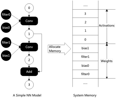
## Diagram: Neural Network Model and Memory Allocation ### Overview This image illustrates the relationship between a computational graph of a simple neural network (left) and its corresponding memory layout in a system (right). The diagram demonstrates how the "Allocate Memory" process maps the network's intermediate data (activations) and parameters (weights/biases) into a structured memory stack. ### Components/Axes **Left Side: A Simple NN Model** * **Nodes (Circles):** Represent data tensors or intermediate states. Labeled 0, 1, 2, 3. * **Operations (Black Rounded Rectangles):** Represent computational layers. Labeled "Conv" (x2) and "Add". * **Parameters (Black Circles):** Represent model weights and biases. Labeled "filter0", "bias0", "filter1", "bias1". * **Flow:** Directed arrows indicate the flow of data. * A skip connection exists from node "1" directly to the "Add" operation. **Middle: Process** * **Arrow:** A large horizontal arrow pointing from the NN Model to the System Memory, labeled "Allocate Memory". **Right Side: System Memory** * **Structure:** A vertical stack representing memory addresses. * **Sections:** * **Activations:** The top portion of the stack. * **Weights:** The bottom portion of the stack. * **Labels:** * Activations: 3, 2, 1, 0 (ordered top to bottom). * Weights: bias1, filter1, bias0, filter0 (ordered top to bottom). * **Ellipses (...):** Located at the very top and very bottom of the memory stack, indicating that the memory continues beyond the shown segment. ### Detailed Analysis **1. NN Model Flow (Left):** * **Input:** Node "0" enters the first "Conv" layer. * **Layer 1:** The first "Conv" layer takes inputs from "filter0" and "bias0". The output is node "1". * **Layer 2:** The second "Conv" layer takes inputs from "filter1" and "bias1", as well as the output from node "1". The output is node "2". * **Final Operation:** The "Add" layer takes inputs from node "2" and node "1" (the skip connection). The final output is node "3". **2. Memory Layout (Right):** * **Activations Region:** This region stores the intermediate tensors generated during the forward pass. The stack contains indices 3, 2, 1, and 0. * **Weights Region:** This region stores the static parameters required for the operations. The stack contains bias1, filter1, bias0, and filter0. * **Spatial Mapping:** The memory is partitioned into two distinct blocks. The "Activations" block is placed above the "Weights" block in this visualization. ### Key Observations * **Parameter Ordering:** The weights are stored in the reverse order of their usage in the computational graph. "filter0" and "bias0" are used in the first layer but are located at the bottom of the "Weights" memory stack. * **Skip Connection:** The diagram explicitly shows a skip connection (from node 1 to the Add operation). This implies that the memory for activation "1" must be retained until the "Add" operation is performed, even after the second "Conv" layer has finished using it. * **Memory Partitioning:** The system clearly distinguishes between dynamic memory (Activations, which change per inference) and static memory (Weights, which are fixed parameters). ### Interpretation This diagram represents the compilation or initialization phase of a neural network inference engine. The "Allocate Memory" step is the critical bridge where the abstract computational graph is transformed into a concrete memory map. The layout suggests a static memory allocation strategy. By pre-allocating memory for all activations (0 through 3) and all weights (filter0/1, bias0/1), the system avoids dynamic memory allocation during the actual inference execution, which is a standard optimization technique in high-performance deep learning frameworks (like TensorRT or TFLite) to reduce latency and prevent memory fragmentation. The inclusion of the skip connection highlights the necessity of managing the lifecycle of activation "1" carefully, as it is required by two different operations at different stages of the graph.