## Scatter Plot Matrix: Evolution of Two Systems (SFC vs. CFC) Over Time
### Overview
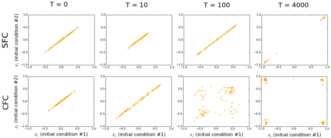
The image displays a 2x4 grid of scatter plots comparing the evolution of two different systems or conditions, labeled "SFC" and "CFC," across four discrete time points (T). Each plot shows the relationship between two variables, `x₁` and `x₂`, which are initialized with specific conditions. The data points are represented as small orange dots.
### Components/Axes
* **Grid Structure:**
* **Rows:** Two rows, labeled on the far left.
* Top Row: **SFC**
* Bottom Row: **CFC**
* **Columns:** Four columns, each with a title at the top indicating the time point.
* Column 1: **T = 0**
* Column 2: **T = 10**
* Column 3: **T = 100**
* Column 4: **T = 4000**
* **Axes (for all subplots):**
* **X-axis:** Labeled `x₁ (initial condition #1)`. The scale runs from -1.0 to 1.0, with major tick marks at -1.0, -0.5, 0.0, 0.5, and 1.0.
* **Y-axis:** Labeled `x₂ (initial condition #2)`. The scale runs from -1.0 to 1.0, with major tick marks at -1.0, -0.5, 0.0, 0.5, and 1.0.
* **Data Series:** A single data series (orange dots) is present in each subplot. There is no separate legend, as the row and column titles provide the necessary categorical context.
### Detailed Analysis
**Row 1: SFC System**
* **T = 0:** Data points form a tight, perfectly linear diagonal from the bottom-left quadrant (~(-0.5, -0.5)) to the top-right quadrant (~(0.5, 0.5)). This indicates a perfect positive correlation between `x₁` and `x₂` at initialization.
* **T = 10:** The linear relationship remains very strong and tight, with minimal dispersion. The line appears slightly shorter, concentrated between approximately -0.4 and 0.4 on both axes.
* **T = 100:** The linear trend persists. The line appears slightly more dispersed than at T=10 but remains clearly defined, stretching from roughly (-0.6, -0.6) to (0.6, 0.6).
* **T = 4000:** The primary linear cluster is still visible, centered around the diagonal. However, a small, distinct cluster of points has appeared in the extreme top-right corner, near (1.0, 1.0). A few isolated points also appear near the bottom-left corner.
**Row 2: CFC System**
* **T = 0:** Identical to the SFC system at T=0. Points form a tight, perfect diagonal line from ~(-0.5, -0.5) to ~(0.5, 0.5).
* **T = 10:** The linear relationship is still dominant but shows slightly more dispersion than the SFC counterpart at the same time. The line spans a similar range.
* **T = 100:** **Significant divergence from the SFC trend.** The data is no longer linear. Points are widely scattered across the plot, forming a diffuse cloud. There is a loose concentration in the central region, but points are present in all quadrants, indicating a breakdown of the initial correlation.
* **T = 4000:** The system has evolved into a highly structured, non-linear state. Data points are tightly clustered in the four corners of the plot: near (-1.0, -1.0), (-1.0, 1.0), (1.0, -1.0), and (1.0, 1.0). Very few points remain near the center or along the original diagonal.
### Key Observations
1. **Identical Initial Conditions:** Both SFC and CFC systems start from the exact same state at T=0—a perfect linear correlation.
2. **Divergent Evolution:** The systems behave identically at T=10 but begin to diverge significantly by T=100.
3. **SFC Stability:** The SFC system largely preserves the initial linear correlation over a very long time (T=4000), with only minor deviations (small clusters at the extremes).
4. **CFC Instability/Phase Transition:** The CFC system undergoes a dramatic transformation. It loses its linear correlation (T=100) and eventually settles into a state where variables `x₁` and `x₂` are driven to their extreme values (+1 or -1), forming four distinct clusters. This suggests a bistable or multi-stable dynamic.
### Interpretation
This visualization likely compares the long-term behavior of two different algorithms, physical models, or dynamical systems (SFC vs. CFC) starting from correlated initial conditions.
* **What the data suggests:** The SFC method appears to be **stable** or **conservative**, maintaining the system's initial structure over time. In contrast, the CFC method is **unstable** or **transformative**, driving the system away from its initial state toward a new, structured equilibrium characterized by extreme values. The corner clusters at T=4000 for CFC are a classic signature of a system with attractors at the boundaries of the state space.
* **How elements relate:** The grid layout is essential for direct comparison. By holding the initial condition (the diagonal line) constant and varying only the system type (SFC/CFC) and time, the plot isolates the effect of the system's governing rules on its evolution.
* **Notable anomalies:** The small cluster at (1.0, 1.0) in the SFC plot at T=4000 is an outlier. It may represent a numerical artifact, a rare trajectory, or the beginning of a very slow instability that would become more pronounced at times beyond T=4000. The complete absence of points along the original diagonal in the CFC plot at T=4000 confirms the total loss of the initial condition's influence.