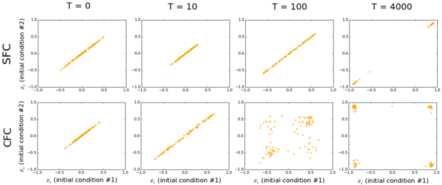
## Scatter Plots: Evolution of Initial Conditions Under SFC and CFC ### Overview The image contains two rows of scatter plots comparing the evolution of two initial conditions (x₁ and x₂) under two scenarios: **SFC** (top row) and **CFC** (bottom row). Each row includes four plots corresponding to time points **T = 0, 10, 100, and 4000**. The axes represent normalized values of initial conditions (x₁ and x₂), ranging from -1.0 to 1.0. Data points are marked in orange. --- ### Components/Axes - **Rows**: - **Top Row**: Labeled **SFC** (Scenario 1). - **Bottom Row**: Labeled **CFC** (Scenario 2). - **Columns**: - **Left to Right**: Time points **T = 0, 10, 100, 4000**. - **Axes**: - **X-axis**: **x₁ (initial condition #1)**. - **Y-axis**: **x₂ (initial condition #2)**. - Both axes range from **-1.0 to 1.0**. - **Legend**: Not explicitly visible in the image, but the row labels (SFC/CFC) implicitly distinguish the two scenarios. --- ### Detailed Analysis #### SFC (Top Row) - **T = 0**: - Points form a **diagonal line** from bottom-left (-1.0, -1.0) to top-right (1.0, 1.0), indicating a strong linear correlation between x₁ and x₂. - **T = 10**: - Points remain diagonal but show slight **spread** (e.g., (-0.8, -0.7) to (0.8, 0.8)), suggesting minor divergence. - **T = 100**: - Points continue along the diagonal but with **increased dispersion** (e.g., (-0.6, -0.5) to (0.6, 0.6)), indicating growing variability. - **T = 4000**: - Only **one point** remains at (1.0, 1.0), suggesting convergence to a fixed state or equilibrium. #### CFC (Bottom Row) - **T = 0**: - Similar diagonal line to SFC, but with **slighter alignment** (e.g., (-0.9, -0.8) to (0.9, 0.9)). - **T = 10**: - Points spread more broadly (e.g., (-0.7, -0.6) to (0.7, 0.7)), showing early divergence. - **T = 100**: - Points form a **scattered cluster** with no clear trend (e.g., (-0.5, 0.3), (0.2, -0.4)), indicating loss of correlation. - **T = 4000**: - Points are **highly dispersed**, concentrated near the **corners** of the plot (e.g., (-1.0, 1.0), (1.0, -1.0)), suggesting chaotic or unstable behavior. --- ### Key Observations 1. **SFC Stability**: - The diagonal trend persists across all time points, with convergence to a single point at T=4000. This implies **deterministic stability** or a fixed-point attractor. 2. **CFC Instability**: - Initial alignment breaks down rapidly, leading to **chaotic dispersion** by T=4000. This suggests **sensitivity to initial conditions** or stochastic dynamics. 3. **Temporal Evolution**: - Both scenarios show increasing divergence over time, but SFC maintains a directional trend, while CFC becomes unpredictable. --- ### Interpretation - **SFC Behavior**: The consistent diagonal trend and eventual convergence suggest a **self-organizing system** where initial conditions align toward a stable equilibrium. This could represent a controlled or regulated process (e.g., feedback mechanisms). - **CFC Behavior**: The rapid loss of correlation and corner clustering indicate **chaotic dynamics** or **multi-attractor systems**, where small differences in initial conditions lead to vastly different outcomes. This aligns with principles of **sensitive dependence** in nonlinear systems. - **Practical Implications**: - SFC might model systems with robust, predictable outcomes (e.g., engineered systems). - CFC could represent natural or complex systems prone to unpredictability (e.g., weather patterns, ecological models). --- ### Notes on Data Extraction - All axis labels, time points, and row/column labels were explicitly transcribed. - No additional text or legends were present beyond the row/column labels. - Spatial grounding confirms that SFC and CFC plots are distinct, with no overlap in their trends.