\n
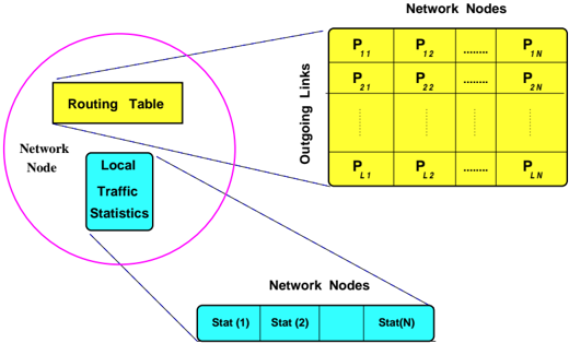
## Diagram: Network Node Internal Structure and Data Flow
### Overview
The image is a conceptual diagram illustrating the internal components of a generic "Network Node" and its data relationships with broader network structures. It uses a color-coded scheme (yellow for routing-related elements, cyan for statistics-related elements) and connecting lines to show information flow. The diagram is schematic and does not contain numerical data or quantitative trends.
### Components/Axes
The diagram is divided into three main spatial regions:
1. **Left Region (Primary Focus):** A large pink circle labeled **"Network Node"**. Inside this circle are two primary components:
* A yellow rectangle labeled **"Routing Table"**.
* A cyan rectangle labeled **"Local Traffic Statistics"**.
2. **Top-Right Region:** A large yellow grid labeled **"Network Nodes"** at the top. The grid is structured as a matrix:
* **Rows:** Labeled on the left side as **"Outgoing Links"**. There are `L` rows, indexed from 1 to `L`.
* **Columns:** Represent different destination network nodes, indexed from 1 to `N`.
* **Cell Content:** Each cell contains a label `P` with two subscripts, `P_ij`, where `i` is the row (link) index and `j` is the column (node) index. The grid shows the first two rows (`P_11, P_12, ..., P_1N` and `P_21, P_22, ..., P_2N`) and the last row (`P_L1, P_L2, ..., P_LN`), with vertical ellipses (`⋮`) indicating intermediate rows.
3. **Bottom-Right Region:** A horizontal cyan bar labeled **"Network Nodes"** above it. This bar is segmented into cells labeled **"Stat (1)"**, **"Stat (2)"**, ..., **"Stat(N)"**.
**Connections (Lines):**
* A line connects the **"Routing Table"** (inside the node) to the top-left corner of the yellow **"Network Nodes"** grid.
* A line connects the **"Local Traffic Statistics"** (inside the node) to the left side of the cyan **"Network Nodes"** statistics bar.
### Detailed Analysis
* **Routing Table Component:** The yellow "Routing Table" is depicted as the source of information that populates or defines the larger yellow matrix. The matrix represents routing parameters (denoted by `P`) for each combination of an outgoing link (`i`) and a destination network node (`j`). The notation `P_ij` strongly suggests these are probabilities, costs, or weights associated with sending traffic from link `i` to node `j`.
* **Local Traffic Statistics Component:** The cyan "Local Traffic Statistics" component is shown as the source for the segmented statistics bar. This implies that local data collected at the individual node is aggregated or reported into a broader set of statistics (`Stat(1)` to `Stat(N)`), likely corresponding to metrics for each of the `N` network nodes.
* **Spatial Grounding:** The legend is effectively the color coding itself: **Yellow** = Routing/Forwarding Plane, **Cyan** = Statistics/Monitoring Plane. The primary "Network Node" circle (pink) acts as a container, isolating the node's internal functions from the external network-wide data structures (the grid and the stats bar) it interacts with.
### Key Observations
1. **Dual-Function Node:** The diagram explicitly separates a network node's function into two distinct planes: a **routing decision plane** (yellow) and a **traffic monitoring plane** (cyan).
2. **Matrix Representation of Routing:** The routing information is not shown as a simple list but as a 2D matrix (`L` links x `N` nodes), indicating a comprehensive mapping of next-hop choices for all possible destinations across all available interfaces.
3. **Aggregation of Statistics:** The "Local Traffic Statistics" do not remain local; they feed into a network-wide view, as shown by the connection to the bar containing statistics for all `N` nodes.
4. **Abstract Notation:** The use of variables (`L`, `N`, `i`, `j`, `P`, `Stat`) instead of concrete numbers indicates this is a general model applicable to networks of varying sizes and topologies.
### Interpretation
This diagram provides a **Peircean investigative** model of a network node's role within a larger system. It moves beyond a simple "black box" view to expose the internal logic:
* **What it demonstrates:** It illustrates the fundamental separation of concerns in network element design. The node must simultaneously solve two problems: **"Where do I send packets?"** (handled by the Routing Table and its matrix of `P_ij` values) and **"What is happening on the network?"** (handled by Local Traffic Statistics, which are aggregated for network-wide analysis).
* **How elements relate:** The flow is cyclical and interdependent. The routing decisions (influenced by the `P_ij` matrix) directly generate the traffic patterns that are then measured by the statistics module. Conversely, the aggregated statistics (`Stat(1)...Stat(N)`) are likely used as input to update or optimize the routing table's `P_ij` values in a real system, creating a feedback loop for adaptive routing.
* **Notable Anomalies/Insights:** The diagram's most significant insight is the **explicit visual linkage between local action and global state**. The line from "Local Traffic Statistics" to the network-wide statistics bar is a powerful representation of how distributed systems build a collective understanding from local observations. The absence of a direct line from the statistics back to the routing table within the node is notable; it suggests that in this model, routing updates might be computed centrally or through a distributed protocol that uses the aggregated statistics as input, rather than being a purely local, autonomous adjustment.