## 2D Scatter/Line Plot: State Estimation Trajectory
### Overview
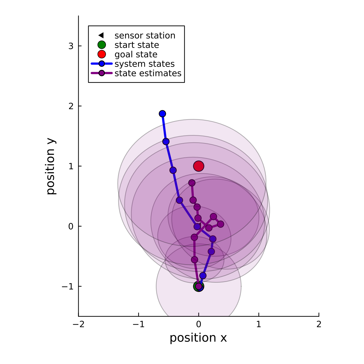
This image displays a 2D Cartesian plot representing a state estimation scenario, likely from a control theory or robotics context (e.g., a Kalman Filter visualization). It compares the "system states" (the ground truth trajectory) against "state estimates" (the filter's belief). The plot includes a start state, a goal state, and uncertainty regions (covariance ellipses) surrounding the state estimates.
### Components/Axes
* **X-axis:** Labeled "position x". The scale ranges from -2 to 2, with major ticks at integer intervals.
* **Y-axis:** Labeled "position y". The scale ranges from -1 to 3, with major ticks at integer intervals.
* **Legend (Top-Left):**
* **Black triangle:** Labeled "sensor station" (Note: This element is absent from the plot area).
* **Green circle:** Labeled "start state".
* **Red circle:** Labeled "goal state".
* **Blue line with blue circles:** Labeled "system states".
* **Purple line with purple circles:** Labeled "state estimates".
* **Uncertainty Regions:** Large, semi-transparent, concentric purple circles centered on the purple "state estimates" markers.
### Detailed Analysis
#### 1. Start and Goal States
* **Start State:** Located at coordinates (0, -1). Marked with a green circle.
* **Goal State:** Located at coordinates (0, 1). Marked with a red circle.
#### 2. System States (Blue Line)
* **Trend:** The blue line represents the actual trajectory of the system. It originates at the start state (0, -1) and moves generally upward and to the left, diverging from the vertical axis.
* **Data Points (Approximate):**
* (0, -1) [Start]
* (-0.5, -0.8)
* (-0.6, -0.4)
* (-0.4, 0.4)
* (-0.5, 0.9)
* (-0.6, 1.4)
* (-0.6, 1.9) [End]
#### 3. State Estimates (Purple Line)
* **Trend:** The purple line represents the estimated trajectory. It originates at the start state (0, -1) and moves generally upward and slightly to the right, before oscillating and clustering near the center.
* **Data Points (Approximate):**
* (0, -1) [Start]
* (0, -0.8)
* (0, -0.6)
* (0, -0.2)
* (0, 0)
* (0.2, -0.2)
* (0.3, 0.1)
* (0.2, 0.1)
* (0.1, 0.3)
* (0.1, 0.4)
* (0.1, 0.7)
* (0, 0.7) [End]
#### 4. Uncertainty Regions
* The purple circles represent the uncertainty (covariance) of the state estimates.
* The circles are largest in the middle of the trajectory (around y=0 to y=0.5), indicating higher uncertainty in the estimate during that phase.
* The circles are smaller near the start state (0, -1) and the end of the purple path (0, 0.7), indicating higher confidence in the estimate at those points.
### Key Observations
* **Divergence:** There is a significant and increasing divergence between the "system states" (blue) and the "state estimates" (purple). The system moves into the top-left quadrant, while the estimates remain clustered near the center-top.
* **Goal Proximity:** The state estimates (purple) appear to be converging toward the "goal state" (red circle at 0, 1), whereas the actual system states (blue) are moving away from the goal toward the top-left.
* **Missing Data:** The legend includes a "sensor station" (black triangle), but no such marker is visible anywhere on the plot. This suggests either an error in the visualization generation or that the sensor station is located outside the plotted bounds.
### Interpretation
This visualization demonstrates a state estimation process where the filter is failing to accurately track the true system state.
* **Filter Performance:** The "state estimates" (purple) are clearly not tracking the "system states" (blue). The filter appears to be "attracted" to the goal state (red), or perhaps the system is moving in a way that the filter's internal model does not account for (e.g., unmodeled dynamics or external disturbances).
* **Uncertainty Analysis:** The large, overlapping purple circles indicate that the filter is aware of its high uncertainty during the middle of the trajectory. The fact that the uncertainty remains large even as the estimates diverge from the true path suggests the filter may be under-confident or that the measurement noise is high.
* **Peircean Investigative Note:** The absence of the "sensor station" is a critical anomaly. If the sensor station is the source of the data for the state estimates, its absence might explain the poor tracking performance—perhaps the sensor is out of range or the data is not being received, leading the filter to rely on a default model that drifts toward the goal.