## Diagram: Convolutional Neural Network Architecture Transformation ### Overview The image depicts a transformation in a convolutional neural network (CNN) architecture. The left side shows a simple sequential structure, while the right side illustrates a more complex, branched architecture, possibly representing an Inception-like module. The diagram uses blocks to represent layers and arrows to indicate the flow of data. ### Components/Axes * **Input (Left):** Black rounded rectangle labeled "input" with dimensions "2x32x40x60". * **Conv (Left):** White rounded rectangle labeled "Conv" with dimensions "2x32x40x60". This appears twice in sequence. * **Add (Left):** White rounded rectangle labeled "Add" with dimensions "2x32x40x60". * **Output (Left):** Black rounded rectangle labeled "output" with dimensions "2x32x40x60". * **Arrow:** A right-pointing arrow indicates the transformation from the left architecture to the right architecture. * **Input (Right):** Black rounded rectangle labeled "input" with dimensions "2x32x40x60". * **Conv (Right):** White rounded rectangles labeled "Conv" with varying dimensions: "1x32x21x60" (appears twice), and other unlabeled "Conv" blocks. * **Add (Right):** White rounded rectangles labeled "Add" with dimensions "1x32x20x60" (appears twice), and other unlabeled "Add" blocks. * **Output (Right):** Black rounded rectangle labeled "output" with dimensions "2x32x40x60". * **Branching Connections (Right):** The right side shows the input splitting into multiple parallel convolutional paths, which are then concatenated via addition operations before producing the final output. * **Dimension Labels:** Dimensions are indicated above the connections between the input and the first layer of Conv blocks on the right side: "1x32x22x60" (appears twice). ### Detailed Analysis **Left Side (Sequential Architecture):** 1. **Input:** The input layer has dimensions 2x32x40x60. 2. **Conv Layer 1:** A convolutional layer with dimensions 2x32x40x60 follows the input. 3. **Conv Layer 2:** Another convolutional layer with dimensions 2x32x40x60 follows the first convolutional layer. 4. **Add Layer:** An addition layer with dimensions 2x32x40x60 combines the output of the second convolutional layer. 5. **Output:** The output layer has dimensions 2x32x40x60. **Right Side (Branched Architecture):** 1. **Input:** The input layer has dimensions 2x32x40x60. 2. **Branching:** The input splits into multiple paths. Two paths are explicitly labeled with dimensions "1x32x22x60". 3. **Convolutional Paths:** * Path 1: Conv (1x32x21x60) -> Conv (1x32x20x60) -> Add (1x32x20x60) * Path 2: Conv (1x32x21x60) -> Conv (1x32x20x60) -> Add (1x32x20x60) * Path 3: Conv -> Conv -> Add * Path 4: Conv -> Conv -> Add 4. **Addition Layers:** The outputs of the convolutional paths are combined using addition layers. 5. **Output:** The output layer has dimensions 2x32x40x60. ### Key Observations * The diagram illustrates a transformation from a simple sequential CNN architecture to a more complex branched architecture. * The branched architecture on the right side resembles an Inception module, where the input is processed through multiple parallel convolutional paths with different filter sizes. * The dimensions of the layers change as the data flows through the network, indicating the application of convolutional operations and pooling. * The addition layers likely serve to concatenate the outputs of the different convolutional paths. ### Interpretation The diagram demonstrates a common technique in CNN design: replacing a simple sequential structure with a more complex, branched structure to improve feature extraction and model performance. The Inception-like module on the right side allows the network to learn features at multiple scales, which can be beneficial for tasks such as image classification and object detection. The transformation suggests an optimization or evolution of the network architecture to enhance its capabilities. The change in dimensions from 2x32x40x60 to 1x32x22x60 and subsequent changes in the branched paths indicate the use of different filter sizes and strides in the convolutional layers. The addition layers likely combine the feature maps learned by the different convolutional paths, allowing the network to integrate information from multiple scales.

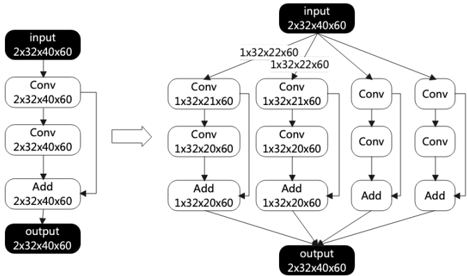
## Diagram: Neural Network Architecture Comparison ### Overview The image displays a comparative diagram of two neural network architectural blocks. The left side depicts a standard residual block, while the right side depicts a multi-branch (parallel) residual architecture. The diagram illustrates the flow of data through these blocks, including tensor shape transformations at each stage. ### Components * **Black Boxes:** Represent the `input` and `output` tensors. * **White Rounded Rectangles:** Represent operational layers, specifically `Conv` (Convolutional) and `Add` (Addition/Residual connection). * **Arrows:** Represent the direction of data flow. * **Text Labels:** Indicate the tensor dimensions (e.g., `2x32x40x60`) at various stages of the network. ### Detailed Analysis #### Left-Hand Side: Standard Residual Block * **Input:** A black box labeled `input` with dimensions `2x32x40x60`. * **Processing:** * The data flows into a `Conv` layer (`2x32x40x60`). * The data flows into a second `Conv` layer (`2x32x40x60`). * A skip connection (the line on the right) bypasses the two `Conv` layers and connects to an `Add` layer. * The `Add` layer combines the output of the second `Conv` layer and the skip connection, resulting in `2x32x40x60`. * **Output:** A black box labeled `output` with dimensions `2x32x40x60`. #### Right-Hand Side: Multi-Branch Residual Architecture * **Input:** A black box labeled `input` with dimensions `2x32x40x60`. * **Branching:** The input splits into four parallel branches. * **Branch 1 & 2 (Leftmost branches):** * The input line is labeled `1x32x22x60`. * The first `Conv` layer has dimensions `1x32x21x60`. * The second `Conv` layer has dimensions `1x32x20x60`. * The `Add` layer has dimensions `1x32x20x60`. * A skip connection bypasses the two `Conv` layers. * **Branch 3 & 4 (Rightmost branches):** * These branches are structurally identical to branches 1 and 2, containing two `Conv` layers and one `Add` layer, but they lack explicit text labels for the tensor dimensions. * **Convergence:** All four branches converge into a single black box labeled `output` with dimensions `2x32x40x60`. ### Key Observations * **Dimensionality Reduction:** In the multi-branch architecture, the branches reduce the spatial dimension from 40 to 20 (as seen in the `1x32x20x60` labels). * **Structural Symmetry:** The right-hand diagram is highly symmetrical, utilizing four identical parallel paths. * **Output Restoration:** Despite the internal reduction in dimensions within the branches, the final output of the multi-branch architecture is `2x32x40x60`, which is identical to the input shape. This implies that the branches are likely concatenated or aggregated in a way that restores the original spatial resolution. * **Missing Labels:** Branches 3 and 4 on the right side are structurally identical to branches 1 and 2 but do not contain the specific tensor dimension text, suggesting they follow the same mathematical transformation. ### Interpretation This diagram illustrates a transition from a standard residual block to a more complex, parallelized architecture, likely inspired by designs such as **ResNeXt** or **Inception** modules. * **The "Split-Transform-Merge" Strategy:** The right-hand side demonstrates a "split-transform-merge" strategy. By splitting the input into four branches, the network can learn different features in parallel. * **Feature Extraction:** The change in dimensions (from 40 to 20) within the branches suggests that the network is performing downsampling or feature extraction at a different scale before merging the results back together. * **Efficiency and Capacity:** The multi-branch approach typically allows for a wider network (more parameters/features) without necessarily increasing the depth linearly, which can improve the representational power of the model while maintaining the original input/output spatial resolution. The skip connections in every branch ensure that the gradient can flow easily through the network, mitigating the vanishing gradient problem.

## Residual Network Block Diagram: Architecture Overview ### Overview The diagram illustrates a residual network (ResNet) block architecture, showing the flow of data through convolutional layers, addition operations, and dimensional transformations. The structure emphasizes skip connections (shortcut paths) that merge with expanded feature maps to produce the final output. ### Components/Axes - **Input**: `2x32x40x60` (batch size, channels, height, width) - **Conv Layers**: - Left path: Two `Conv` operations maintaining `2x32x40x60` dimensions. - Right path: Four `Conv` operations with decreasing spatial dimensions: - `1x32x22x60` → `1x32x20x60` (via two `Conv` layers). - **Add Operations**: Element-wise addition of feature maps. - **Output**: `2x32x40x60` (matches input dimensions via skip connection). ### Detailed Analysis 1. **Left Path (Shortcut)**: - Input → `Conv(2x32x40x60)` → `Conv(2x32x40x60)` → `Add` → Output. - Dimensions remain unchanged via identity mapping. 2. **Right Path (Expansion)**: - Input splits into four branches: - **Branch 1**: `Conv(1x32x22x60)` → `Conv(1x32x20x60)` → `Add` → `1x32x20x60`. - **Branch 2**: `Conv(1x32x22x60)` → `Conv(1x32x20x60)` → `Add` → `1x32x20x60`. - **Branch 3**: `Conv(1x32x22x60)` → `Conv(1x32x20x60)` → `Add` → `1x32x20x60`. - **Branch 4**: `Conv(1x32x22x60)` → `Conv(1x32x20x60)` → `Add` → `1x32x20x60`. - Branches merge via element-wise addition to produce `1x32x20x60`. 3. **Final Merge**: - Right path output (`1x32x20x60`) is upsampled or transformed (implied but not explicitly labeled) to match the left path's `2x32x40x60` dimensions. - Merged with left path output via `Add` to produce final `2x32x40x60` output. ### Key Observations - **Dimensional Consistency**: The left path preserves input dimensions, while the right path reduces spatial resolution (40→20) but increases channel depth (1→2 via branching). - **Skip Connection**: The identity shortcut ensures gradients flow directly through the network, mitigating vanishing gradient issues. - **Feature Aggregation**: Four parallel `Conv` branches suggest feature diversification before merging. ### Interpretation This ResNet block demonstrates the core innovation of residual networks: **learning residual functions** instead of raw outputs. By adding skip connections, the network learns identity mappings (via the left path) and complex transformations (via the right path), enabling deeper architectures without degradation. The four-branch design on the right likely captures multi-scale features, while the final upsampling (implied) restores spatial resolution for seamless integration with the shortcut path. This architecture is foundational for training very deep networks (e.g., 152+ layers) by balancing depth with gradient stability.