## Histograms: Time Distribution Analysis
### Overview
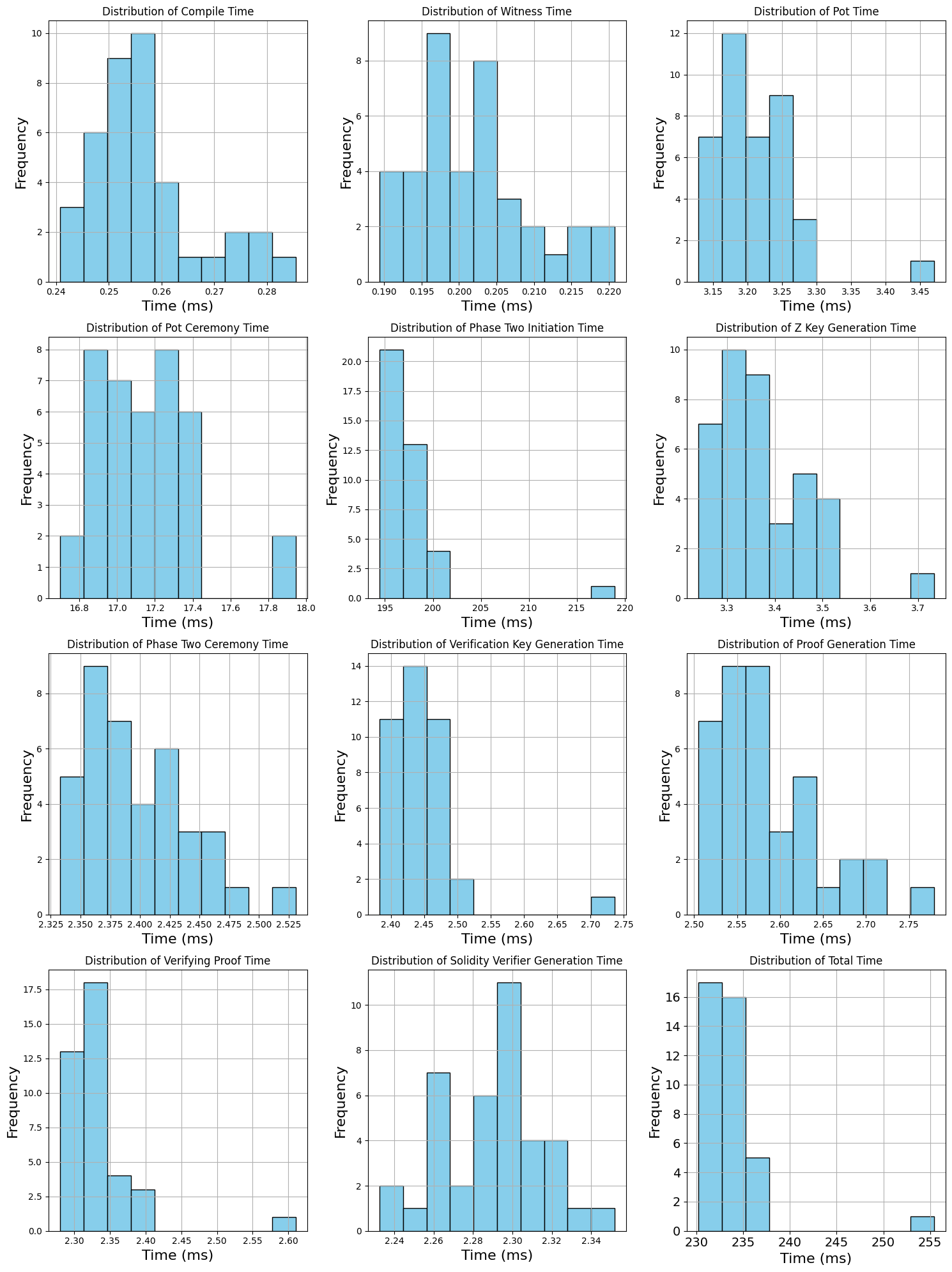
The image contains 12 histograms visualizing time distributions across various computational processes. Each histogram uses a blue bar color scheme with frequency counts on the y-axis and time measurements (in milliseconds) on the x-axis. Titles indicate specific metrics like "Compile Time," "Witness Time," and "Total Time."
---
### Components/Axes
1. **X-Axes**:
- Labeled "Time (ms)" across all charts.
- Ranges vary per metric (e.g., 0.24–0.28 ms for Compile Time, 230–255 ms for Total Time).
2. **Y-Axes**:
- Labeled "Frequency" across all charts.
- Scales range from 0 to ~20 (e.g., 0–12 for Pot Time, 0–20 for Phase Two Initiation Time).
3. **Legends**:
- No explicit legends present; bar colors are uniform (blue) across all charts.
---
### Detailed Analysis
#### Top Row (Left to Right)
1. **Compile Time**
- **X-Axis**: 0.24–0.28 ms
- **Peaks**: ~0.25 ms (frequency ~10), ~0.26 ms (frequency ~4)
- **Tails**: Low frequencies at 0.24 ms and 0.28 ms.
2. **Witness Time**
- **X-Axis**: 0.190–0.220 ms
- **Peaks**: ~0.195 ms (frequency ~10), ~0.205 ms (frequency ~8)
- **Tails**: Gradual decline toward 0.220 ms.
3. **Pot Time**
- **X-Axis**: 3.15–3.45 ms
- **Peaks**: ~3.20 ms (frequency ~12), ~3.25 ms (frequency ~9)
- **Tails**: Sharp drop after 3.30 ms.
#### Middle Row (Left to Right)
4. **Pot Ceremony Time**
- **X-Axis**: 16.8–18.0 ms
- **Peaks**: ~17.0 ms (frequency ~8), ~17.2 ms (frequency ~8)
- **Tails**: Low frequencies at 16.8 ms and 17.8 ms.
5. **Phase Two Initiation Time**
- **X-Axis**: 195–220 ms
- **Peaks**: ~195 ms (frequency ~20), ~200 ms (frequency ~13)
- **Tails**: Sparse data beyond 205 ms.
6. **Z Key Generation Time**
- **X-Axis**: 3.3–3.7 ms
- **Peaks**: ~3.3 ms (frequency ~10), ~3.4 ms (frequency ~9)
- **Tails**: Drop after 3.5 ms.
#### Bottom Row (Left to Right)
7. **Phase Two Ceremony Time**
- **X-Axis**: 2.325–2.525 ms
- **Peaks**: ~2.35 ms (frequency ~9), ~2.425 ms (frequency ~6)
- **Tails**: Gradual decline toward 2.525 ms.
8. **Verification Key Generation Time**
- **X-Axis**: 2.40–2.75 ms
- **Peaks**: ~2.45 ms (frequency ~14), ~2.50 ms (frequency ~11)
- **Tails**: Sharp drop after 2.55 ms.
9. **Proof Generation Time**
- **X-Axis**: 2.50–2.75 ms
- **Peaks**: ~2.55 ms (frequency ~9), ~2.60 ms (frequency ~5)
- **Tails**: Low frequencies at 2.70 ms and 2.75 ms.
#### Final Row (Left to Right)
10. **Verifying Proof Time**
- **X-Axis**: 2.30–2.60 ms
- **Peaks**: ~2.35 ms (frequency ~18), ~2.40 ms (frequency ~13)
- **Tails**: Sparse data at 2.60 ms.
11. **Solidity Verifier Generation Time**
- **X-Axis**: 2.24–2.34 ms
- **Peaks**: ~2.30 ms (frequency ~11), ~2.32 ms (frequency ~10)
- **Tails**: Drop after 2.34 ms.
12. **Total Time**
- **X-Axis**: 230–255 ms
- **Peaks**: ~230 ms (frequency ~17), ~235 ms (frequency ~16)
- **Tails**: Small peak at 255 ms (frequency ~1).
---
### Key Observations
1. **Narrow Distributions**: Most metrics (e.g., Compile Time, Witness Time) show tight clustering around peak values, indicating consistency.
2. **Long-Tail Metrics**: Phase Two Initiation Time and Total Time exhibit longer tails, suggesting occasional outliers or variability.
3. **High-Frequency Peaks**: Metrics like Pot Time (3.20 ms) and Verification Key Generation Time (2.45 ms) have dominant modes.
4. **Anomalies**: The Total Time histogram shows a rare outlier at 255 ms, far from the main cluster.
---
### Interpretation
- **Consistency vs. Variability**: Metrics with narrow distributions (e.g., Compile Time) suggest predictable performance, while those with long tails (e.g., Total Time) indicate potential bottlenecks or external dependencies.
- **Process Hierarchy**: Shorter time metrics (e.g., Witness Time at 0.195 ms) likely represent foundational steps, while longer ones (e.g., Total Time at 230 ms) aggregate multiple processes.
- **Critical Paths**: Phase Two Initiation Time (195–200 ms) and Verification Key Generation Time (2.45 ms) may represent computationally intensive stages requiring optimization.
- **Outlier Implications**: The 255 ms outlier in Total Time could signal edge-case scenarios (e.g., network delays, resource contention) warranting further investigation.
This analysis highlights the importance of optimizing high-frequency peaks and addressing long-tail distributions to improve overall system efficiency.