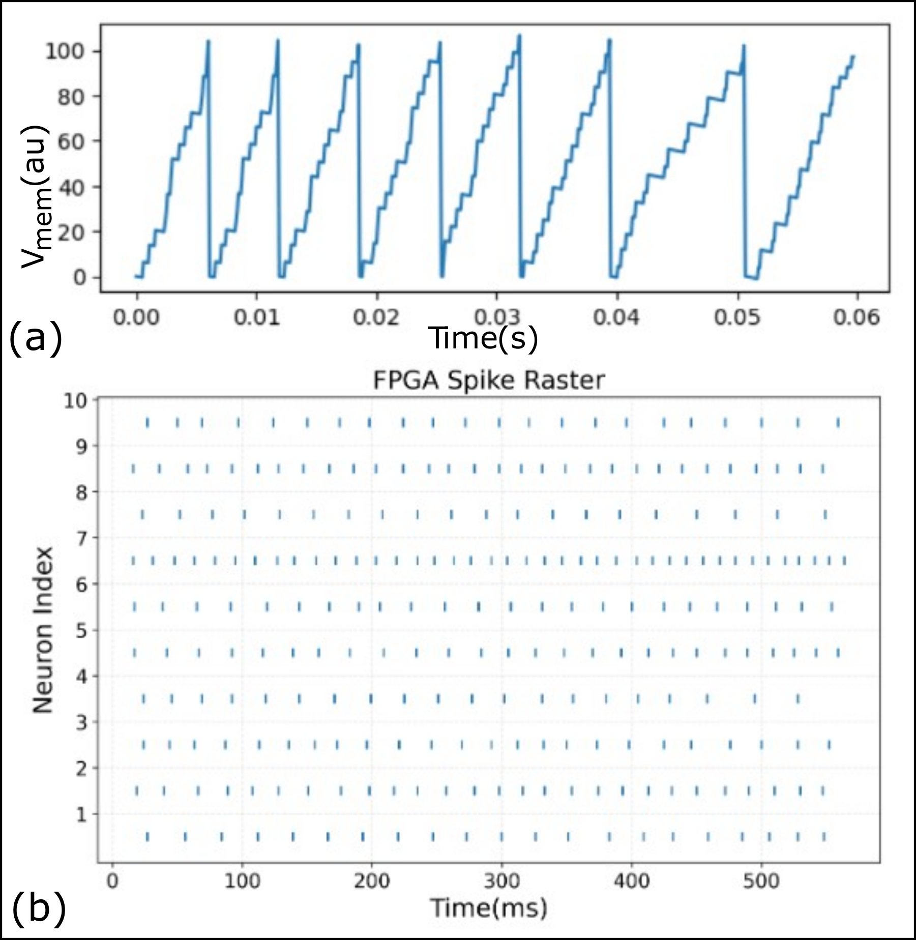
## [Chart/Diagram Type]: Neural Membrane Potential and Spike Raster Plot ### Overview The image contains two vertically stacked subplots, labeled (a) and (b), presenting data from a spiking neural network simulation or hardware implementation (likely on an FPGA). Subplot (a) shows the membrane potential of a single neuron over a short time window. Subplot (b) is a spike raster plot showing the firing times of 10 neurons over a longer duration. The data appears to be from a technical or scientific context, likely related to neuromorphic computing. ### Components/Axes **Subplot (a): Membrane Potential Trace** * **Y-axis:** Label is `Vmem(au)`. "au" stands for arbitrary units. The scale runs from 0 to 100, with major tick marks at 0, 20, 40, 60, 80, and 100. * **X-axis:** Label is `Time(s)`. The scale runs from 0.00 to 0.06 seconds, with major tick marks at 0.00, 0.01, 0.02, 0.03, 0.04, 0.05, and 0.06. * **Data Series:** A single blue line representing the membrane potential (`Vmem`) of one neuron. * **Label:** The subplot is labeled `(a)` in the bottom-left corner, outside the axes. **Subplot (b): Spike Raster Plot** * **Title:** `FPGA Spike Raster` is centered above the plot. * **Y-axis:** Label is `Neuron Index`. The scale runs from 1 to 10, with integer tick marks for each neuron index. * **X-axis:** Label is `Time(ms)`. The scale runs from 0 to 500 milliseconds, with major tick marks at 0, 100, 200, 300, 400, and 500. * **Data Series:** Ten horizontal rows of blue vertical tick marks. Each row corresponds to a neuron (index 1-10), and each tick mark represents a spike event at a specific time. * **Label:** The subplot is labeled `(b)` in the bottom-left corner, outside the axes. ### Detailed Analysis **Subplot (a) Analysis:** * **Trend:** The line exhibits a characteristic "integrate-and-fire" neuron model pattern. It shows a stepwise, approximately linear increase in membrane potential, followed by a near-instantaneous reset to a baseline value (approximately 0 au). This cycle repeats. * **Key Data Points (Approximate):** * **Spike 1:** Rises from ~0 au at t=0.000s to a peak of ~105 au at t≈0.006s, then resets. * **Spike 2:** Rises from ~0 au at t≈0.006s to a peak of ~105 au at t≈0.012s, then resets. * **Spike 3:** Rises from ~0 au at t≈0.012s to a peak of ~105 au at t≈0.018s, then resets. * **Spike 4:** Rises from ~0 au at t≈0.018s to a peak of ~105 au at t≈0.025s, then resets. * **Spike 5:** Rises from ~0 au at t≈0.025s to a peak of ~105 au at t≈0.032s, then resets. * **Spike 6:** Rises from ~0 au at t≈0.032s to a peak of ~105 au at t≈0.039s, then resets. * **Spike 7:** Rises from ~0 au at t≈0.039s to a peak of ~105 au at t≈0.051s, then resets. This inter-spike interval appears slightly longer. * **Spike 8:** Rises from ~0 au at t≈0.051s to ~98 au at t=0.060s (end of plot). * **Pattern:** The inter-spike interval (time between resets) is roughly constant at ~0.006-0.007 seconds, corresponding to a firing frequency of approximately 140-165 Hz. The rise is not perfectly smooth but has a staircase-like appearance, suggesting discrete time steps or digital integration. **Subplot (b) Analysis:** * **Trend:** The plot shows the temporal firing patterns of 10 distinct neurons. The spikes (blue ticks) are distributed across the 500 ms window. * **Neuron-Specific Patterns (Visual Inspection):** * **Neuron 1:** Fires regularly, with spikes spaced roughly 25-30 ms apart. * **Neuron 2:** Fires regularly, similar to Neuron 1. * **Neuron 3:** Fires regularly. * **Neuron 4:** Fires regularly. * **Neuron 5:** Fires regularly. * **Neuron 6:** Appears to have the highest firing rate, with spikes very closely spaced (approximately every 15-20 ms). * **Neuron 7:** Fires regularly. * **Neuron 8:** Fires regularly. * **Neuron 9:** Fires regularly. * **Neuron 10:** Fires regularly. * **Overall Pattern:** All neurons exhibit sustained, relatively regular spiking activity throughout the 500 ms period. There is no obvious synchronization or bursting pattern across the population; each neuron appears to fire independently at its own rate. Neuron 6 is a clear outlier with a significantly higher firing frequency. ### Key Observations 1. **Single-Neuron vs. Population View:** Subplot (a) provides a high-resolution view of the membrane dynamics leading to a single spike, while subplot (b) provides a population-level view of spike timing over a longer period. 2. **Regular Spiking:** Both plots indicate regular spiking behavior. The neuron in (a) has a consistent inter-spike interval, and the neurons in (b) fire at steady, albeit different, rates. 3. **Firing Rate Discrepancy:** The neuron in (a) fires at ~150 Hz. In (b), most neurons appear to fire at a lower rate (e.g., Neuron 1: ~33-40 Hz), while Neuron 6 fires at a much higher rate (~50-67 Hz). This suggests the neuron in (a) may be a different type or under different input conditions than those in (b). 4. **Digital Implementation:** The staircase rise in (a) and the title "FPGA Spike Raster" strongly indicate this is data from a digital, hardware (FPGA-based) implementation of a spiking neural network, not an analog biological recording. 5. **No Explicit Correlation:** There is no visual cue linking a specific spike in (a) to a specific tick in (b). They are presented as complementary views of system behavior. ### Interpretation This figure demonstrates the fundamental operation of a spiking neural network (SNN) implemented on digital hardware (FPGA). * **What the data suggests:** Subplot (a) validates the core neuron model's functionality: it correctly integrates input (stepwise rise) and generates a spike (reset) upon reaching a threshold (~105 au). Subplot (b) confirms that a network of such neurons can sustain asynchronous, ongoing spiking activity, which is the basis for temporal information processing in SNNs. * **How elements relate:** The two plots are causally linked. The membrane potential dynamics shown in (a) are the underlying mechanism that produces each individual spike tick seen in (b). The raster plot is the aggregate output of many such neurons operating in parallel. * **Notable implications:** The regularity of spiking suggests the network might be in a stable state or driven by constant input. The outlier (Neuron 6) could be receiving stronger input, have different synaptic weights, or represent a different neuron type within the network. The use of an FPGA highlights a focus on efficient, low-power, hardware-accelerated neural computation, a key area in neuromorphic engineering. The "arbitrary units" for voltage indicate the focus is on the model's dynamics and timing, not on matching specific biological voltage values.