## [Chart Type]: Dual Line Charts – Cross Sections of a Prior Function
### Overview
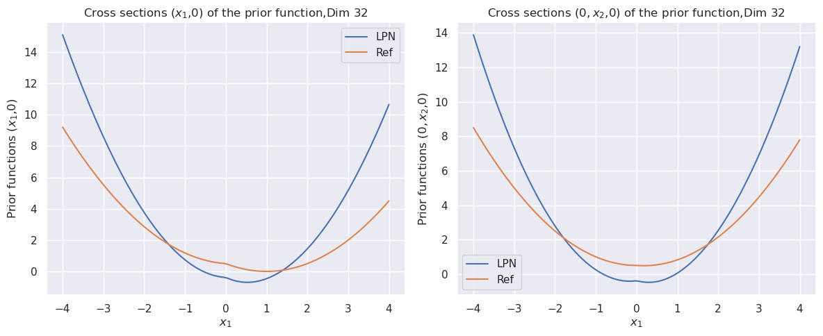
The image displays two side-by-side line charts, each plotting the cross-section of a "prior function" in a 32-dimensional space. The charts compare two functions, labeled "LPN" (blue line) and "Ref" (orange line), across a range of values for a variable labeled `x₁`. The left chart shows the cross-section at `(x₁, 0)`, while the right chart shows the cross-section at `(0, x₂, 0)`. Both charts share identical axes and scales, facilitating direct comparison.
### Components/Axes
* **Titles:**
* Left Chart: `Cross sections (x₁,0) of the prior function,Dim 32`
* Right Chart: `Cross sections (0, x₂,0) of the prior function,Dim 32`
* **X-Axis (Both Charts):**
* Label: `x₁`
* Scale: Linear, ranging from -4 to 4.
* Tick Marks: -4, -3, -2, -1, 0, 1, 2, 3, 4.
* **Y-Axis (Both Charts):**
* Label: `Prior functions (x₁,0)` (left) and `Prior functions (0, x₂,0)` (right).
* Scale: Linear, ranging from 0 to 14.
* Tick Marks: 0, 2, 4, 6, 8, 10, 12, 14.
* **Legend (Both Charts):**
* Position: Top-right corner of each plot area.
* Entries:
* `LPN` (Blue line)
* `Ref` (Orange line)
### Detailed Analysis
Both charts depict U-shaped (parabolic) curves, indicating that the value of the prior function is minimized near `x₁ = 0` and increases as `x₁` moves toward the extremes (-4 or 4).
**Left Chart: Cross-section (x₁, 0)**
* **LPN (Blue Line):**
* **Trend:** Starts at a high value, decreases to a minimum near `x₁ = 0`, then increases symmetrically.
* **Approximate Data Points:**
* At `x₁ = -4`: y ≈ 15.0
* At `x₁ = -2`: y ≈ 4.0
* At `x₁ = 0`: y ≈ -0.5 (Note: The curve dips slightly below the y=0 axis)
* At `x₁ = 2`: y ≈ 4.0
* At `x₁ = 4`: y ≈ 10.5
* **Ref (Orange Line):**
* **Trend:** Follows a similar U-shape but is consistently lower than the LPN curve across the entire range.
* **Approximate Data Points:**
* At `x₁ = -4`: y ≈ 9.2
* At `x₁ = -2`: y ≈ 2.5
* At `x₁ = 0`: y ≈ 0.0
* At `x₁ = 2`: y ≈ 2.5
* At `x₁ = 4`: y ≈ 4.5
**Right Chart: Cross-section (0, x₂, 0)**
* **LPN (Blue Line):**
* **Trend:** Similar U-shape, but the curve appears slightly steeper and the minimum is more pronounced.
* **Approximate Data Points:**
* At `x₁ = -4`: y ≈ 13.8
* At `x₁ = -2`: y ≈ 3.0
* At `x₁ = 0`: y ≈ -0.8 (Note: The minimum is lower than in the left chart)
* At `x₁ = 2`: y ≈ 3.0
* At `x₁ = 4`: y ≈ 13.2
* **Ref (Orange Line):**
* **Trend:** U-shaped, consistently lower than the LPN curve.
* **Approximate Data Points:**
* At `x₁ = -4`: y ≈ 8.5
* At `x₁ = -2`: y ≈ 2.0
* At `x₁ = 0`: y ≈ 0.5
* At `x₁ = 2`: y ≈ 2.0
* At `x₁ = 4`: y ≈ 7.8
### Key Observations
1. **Consistent Hierarchy:** In both cross-sections, the LPN function (blue) yields higher values than the Ref function (orange) for all `x₁` values except possibly at the very minima where they are close.
2. **Symmetry:** Both functions in both charts appear symmetric around `x₁ = 0`.
3. **Minima Location:** The minimum value for both functions occurs at or very near `x₁ = 0`.
4. **Cross-Section Difference:** The LPN curve in the right chart (`(0, x₂, 0)`) has a deeper minimum (≈ -0.8) compared to the left chart (`(x₁, 0)`, ≈ -0.5). The Ref curve's minimum is slightly higher in the right chart (≈ 0.5) compared to the left (≈ 0.0).
5. **Growth Rate:** The LPN function grows more rapidly away from the minimum than the Ref function in both cases.
### Interpretation
These charts visualize and compare the behavior of two prior probability distributions (LPN and Ref) in a high-dimensional (32D) space by taking 1D slices. The U-shape indicates that both priors assign lower probability density (or higher negative log-probability, depending on the function's definition) to values near zero and higher density to values far from zero along these specific axes.
The key finding is that the **LPN prior is consistently "heavier-tailed" or assigns relatively higher density to extreme values** compared to the Ref prior. This is evident because the blue LPN curve is always above the orange Ref curve. In a Bayesian context, this suggests the LPN prior is less informative or more diffuse, allowing data to have a stronger influence on the posterior distribution, especially for parameters far from zero. The difference in the minima between the two cross-sections hints at anisotropy in the prior's shape within the 32-dimensional space—its behavior is not identical in all directions. The charts effectively demonstrate that the choice between LPN and Ref priors would lead to different regularization behaviors in a statistical model.