## Vector Field Diagram: 3D Vector Field Visualization ### Overview The image is a 3D vector field diagram within a rectangular prism. The diagram visualizes a vector field using black arrows, with a blue rectangular plane intersecting the field. The axes are labeled as eA, eB, and eC. ### Components/Axes * **Axes:** * eA: Vertical axis, ranging from 0.99 to 1.01, with a marked value at 1. * eB: Horizontal axis, ranging from -0.01 to 0.01, with a marked value at 0. * eC: Depth axis, ranging from -0.01 to 0.01, with marked values at -0.01, 0, and 0.01. * **Vector Field:** Represented by black arrows indicating direction and magnitude. * **Blue Plane:** A rectangular plane colored blue, intersecting the vector field. The plane is outlined in blue. ### Detailed Analysis or Content Details * **Vector Field Arrows:** The black arrows appear to be generally aligned, flowing from the top-left towards the bottom-right of the prism. * **Blue Plane Vectors:** The arrows on the blue plane are oriented in a consistent direction, generally pointing downwards and slightly to the right. * **Axis Values:** * eA: 0.99, 1, 1.01 * eB: -0.01, 0, 0.01 * eC: -0.01, 0, 0.01 ### Key Observations * The vector field appears relatively uniform outside the blue plane. * The vectors on the blue plane show a consistent direction, suggesting a specific flow pattern within that region. * The axes provide a coordinate system for understanding the spatial distribution of the vector field. ### Interpretation The diagram visualizes a 3D vector field and its interaction with a specific plane. The consistent direction of vectors on the blue plane suggests a defined flow or force acting within that region. The axes provide a reference frame for quantifying the vector field's behavior in 3D space. The diagram could represent a physical phenomenon, such as fluid flow or electromagnetic field, where the blue plane represents a boundary or interface.

\n ## Diagram: Vector Field Visualization ### Overview The image depicts a three-dimensional vector field within a cuboid volume. Arrows represent vectors at various points in space, indicating magnitude and direction. A blue plane is positioned within the volume, intersecting the vector field. The axes are labeled with exponential terms: e^A, e^B, and e^C. ### Components/Axes * **Axes:** * X-axis: e^A, ranging from approximately -0.01 to 1.01. Marked values: -0.01, 0, 1, 1.01 * Y-axis: e^B, ranging from approximately -0.01 to 0.01. Marked values: -0.01, 0, 0.01 * Z-axis: e^C, ranging from approximately -0.01 to 0.01. Marked values: -0.01, 0, 0.01 * **Vectors:** Black arrows distributed throughout the volume, representing the vector field. * **Plane:** A blue, rectangular plane intersecting the vector field. It appears to be aligned with the axes. ### Detailed Analysis The vector field appears to have a consistent direction, generally pointing downwards and slightly to the right (negative e^C and positive e^A). The density of vectors seems relatively uniform throughout the visualized volume. The plane intersects the vectors, providing a visual slice through the field. The vectors within the plane are generally aligned with the overall field direction. The magnitude of the vectors appears to be relatively constant, as the arrow lengths do not vary significantly. ### Key Observations * The vector field is relatively smooth and consistent. * The plane provides a cross-section of the field, allowing for visualization of the vector distribution. * The axes are scaled using exponential functions, which may indicate a non-linear relationship between the coordinates and the physical space they represent. * The values on the axes are very small, suggesting a zoomed-in view of a larger system. ### Interpretation This diagram likely represents a simplified model of a physical phenomenon described by a vector field. The exponential scaling of the axes suggests that the underlying system may be sensitive to small changes in the coordinates. The consistent direction of the vectors indicates a dominant force or gradient driving the field. The plane could represent a boundary or a specific region of interest within the system. The visualization allows for qualitative assessment of the field's behavior within that region. The diagram doesn't provide specific numerical data beyond the axis labels, so a quantitative analysis is not possible. However, the visual representation suggests a stable and predictable system, with a well-defined vector field. The choice of exponential axes is notable and suggests the underlying mathematical model involves exponential functions. This could represent growth, decay, or other exponential processes.

## 3D Vector Field Diagram: Convergence to a Plane ### Overview The image displays a three-dimensional vector field plot contained within a wireframe box. The plot visualizes a directional flow (represented by black arrows) within a defined volume of space. A prominent, semi-transparent blue plane cuts diagonally through this volume, and the vector field appears to converge toward this plane from both sides. ### Components/Axes * **Coordinate System:** A 3D Cartesian coordinate system is depicted with three orthogonal axes. * **Axis Labels & Ranges:** * **e^A (Vertical Axis):** Labeled on the left side. The scale runs from **0.99** at the bottom to **1.01** at the top. The midpoint tick is labeled **1**. * **e^B (Horizontal Axis, front):** Labeled along the bottom front edge. The scale runs from **-0.01** on the left to **0.01** on the right. The midpoint tick is labeled **0**. * **e^C (Depth Axis, right side):** Labeled on the right side. The scale runs from **-0.01** at the bottom to **0.01** at the top. The midpoint tick is labeled **0**. * **Key Geometric Element:** A **blue, semi-transparent plane** is positioned diagonally within the volume. It is bounded by a blue outline. Its orientation suggests it is defined by a relationship between the e^A, e^B, and e^C variables. * **Vector Field:** Numerous **black arrows** are distributed throughout the volume. Each arrow has a shaft and an arrowhead indicating direction. ### Detailed Analysis * **Vector Field Behavior:** The arrows exhibit a uniform, laminar flow pattern. Their primary direction is **toward the blue plane**. * Arrows located "above" the plane (in the region of higher e^A) point downward and inward toward the plane. * Arrows located "below" the plane (in the region of lower e^A) point upward and inward toward the plane. * The flow appears symmetric and convergent from both sides of the plane. * **Spatial Grounding of the Blue Plane:** The plane is positioned such that it intersects the e^A axis at approximately **e^A = 1**. It is tilted, meaning its intersection with the e^B-e^C plane is a line, not a point. The plane's orientation suggests a linear relationship, likely of the form `e^A = 1 + k1*e^B + k2*e^C` for some constants k1 and k2. * **Data Point Confirmation:** There are no discrete data points or plotted series. The information is conveyed entirely through the continuous vector field and the reference plane. ### Key Observations 1. **Convergence:** The most salient feature is the convergence of the vector field onto the blue plane. This indicates the plane represents a set of equilibrium points or a stable manifold for the system being visualized. 2. **Narrow Parameter Range:** The axes are zoomed in on a very small region of state space (e^A within ±0.01 of 1, e^B and e^C within ±0.01 of 0). This suggests the analysis is focused on local behavior near the point (e^A=1, e^B=0, e^C=0). 3. **Uniformity:** The vector field appears highly regular and uniform in direction and magnitude (as implied by arrow length) across the displayed volume, suggesting a linear or linearized system. 4. **Diagonal Attractor:** The attractor (the blue plane) is not aligned with any primary axis, indicating the stable dynamics involve a coupled relationship between all three variables (e^A, e^B, e^C). ### Interpretation This diagram is a technical visualization likely from the fields of dynamical systems, control theory, or stability analysis. It depicts the **local stability** of a system around an equilibrium point located at (e^A=1, e^B=0, e^C=0). * **What the data suggests:** The vector field shows the instantaneous direction of change for any state within this volume. The consistent flow toward the blue plane demonstrates that if the system is perturbed away from this plane, its dynamics will drive it back toward it. Therefore, the blue plane is a **stable equilibrium manifold**. * **Relationship between elements:** The axes define the state space variables. The vector field defines the system's governing laws (e.g., differential equations). The blue plane is a geometric representation of the solution set where the system's rate of change is zero (an equilibrium). The convergence of vectors onto it visually proves its stability. * **Notable implications:** The fact that the attractor is a plane (a 2D surface) within a 3D space, rather than a single point, indicates the system has a **conserved quantity** or a **zero eigenvalue** in its linearization. There is one direction (perpendicular to the plane) in which the system is stable, and two directions (within the plane) where it is neutrally stable or marginally stable. The narrow axis ranges confirm this is a **local analysis**; the global behavior could be different.

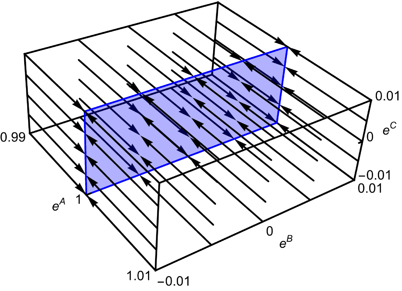
## 3D Vector Field Diagram: Central Region Analysis ### Overview The image depicts a 3D coordinate system with axes labeled **e^A**, **e^B**, and **e^C**. A semi-transparent blue shaded region occupies the central space, surrounded by black arrows with blue tips pointing in various directions. The axes are scaled with approximate numerical values, and the diagram emphasizes directional relationships within the shaded region. --- ### Components/Axes 1. **Axes Labels and Scales**: - **e^A Axis**: - Range: **0.99 to 1.01** (centered at 1.00). - Position: Leftmost axis, oriented diagonally in the 3D space. - **e^B Axis**: - Range: **-0.01 to 0.01** (centered at 0). - Position: Bottom axis, horizontal in the 3D space. - **e^C Axis**: - Range: **-0.01 to 0.01** (centered at 0). - Position: Rightmost axis, vertical in the 3D space. 2. **Blue Shaded Region**: - A rectangular prism centered at **(e^A=1.00, e^B=0, e^C=0)**. - Dimensions: Spans the full range of **e^A** (0.99–1.01) and partial ranges of **e^B** and **e^C** (-0.01–0.01). - Transparency: Semi-transparent, suggesting a gradient or intensity variation. 3. **Arrows**: - Black vectors with blue tips distributed throughout the 3D space. - Directions: Point toward or away from the blue shaded region, indicating flow, influence, or interaction. - Density: Higher concentration near the blue region, suggesting localized activity. --- ### Detailed Analysis - **Axis Values**: - **e^A**: Dominates the scale (0.99–1.01), with the blue region anchored at **e^A=1.00**. - **e^B and e^C**: Narrower ranges (-0.01–0.01), indicating secondary variables with minimal variation. - **Blue Region**: - Positioned at the intersection of **e^A=1.00**, **e^B=0**, and **e^C=0**. - Likely represents a critical threshold or equilibrium point in the system. - **Arrows**: - Orientations vary: Some point radially outward from the blue region, others inward or tangential. - Suggests dynamic interactions (e.g., forces, gradients) centered on the shaded area. --- ### Key Observations 1. **Central Focus**: The blue region is spatially and numerically centered at **(1.00, 0, 0)**, emphasizing its significance. 2. **Axis Dominance**: **e^A** has the largest scale, while **e^B** and **e^C** are tightly constrained, implying their roles as secondary parameters. 3. **Arrow Dynamics**: Arrows near the blue region point in divergent directions, hinting at competing or interacting forces. 4. **Transparency Gradient**: The blue region’s semi-transparency may indicate a decay or diffusion effect from the center. --- ### Interpretation - **System Behavior**: The diagram likely models a physical or mathematical system where **e^A=1.00** is a critical state (e.g., phase transition, resonance). The blue region represents this state, with arrows visualizing perturbations or influences around it. - **Directional Relationships**: Arrows pointing toward the blue region could signify attraction or convergence, while outward-pointing arrows might represent divergence or instability. - **Scale Implications**: The narrow ranges of **e^B** and **e^C** suggest these variables are tightly controlled or have minimal impact compared to **e^A**. - **Anomalies**: No outliers are visible, but the uniform arrow distribution implies a homogeneous field outside the blue region. --- ### Conclusion This diagram illustrates a 3D vector field centered on a critical threshold (**e^A=1.00**), with directional interactions concentrated in the blue-shaded region. The axes and arrows collectively highlight the dominance of **e^A** and the dynamic interplay of forces within the system. The absence of a legend leaves the exact nature of the vectors open to interpretation, but their spatial distribution strongly suggests a focus on the central equilibrium point.