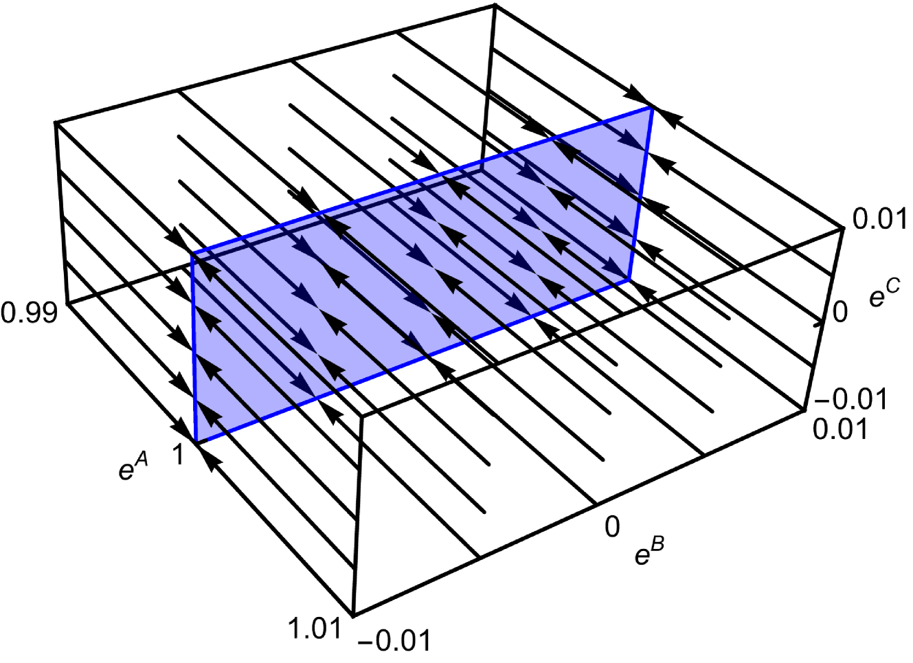
\n ## Diagram: Vector Field Visualization ### Overview The image depicts a three-dimensional vector field within a cuboid volume. Arrows represent vectors at various points in space, indicating magnitude and direction. A blue plane is positioned within the volume, intersecting the vector field. The axes are labeled with exponential terms: e^A, e^B, and e^C. ### Components/Axes * **Axes:** * X-axis: e^A, ranging from approximately -0.01 to 1.01. Marked values: -0.01, 0, 1, 1.01 * Y-axis: e^B, ranging from approximately -0.01 to 0.01. Marked values: -0.01, 0, 0.01 * Z-axis: e^C, ranging from approximately -0.01 to 0.01. Marked values: -0.01, 0, 0.01 * **Vectors:** Black arrows distributed throughout the volume, representing the vector field. * **Plane:** A blue, rectangular plane intersecting the vector field. It appears to be aligned with the axes. ### Detailed Analysis The vector field appears to have a consistent direction, generally pointing downwards and slightly to the right (negative e^C and positive e^A). The density of vectors seems relatively uniform throughout the visualized volume. The plane intersects the vectors, providing a visual slice through the field. The vectors within the plane are generally aligned with the overall field direction. The magnitude of the vectors appears to be relatively constant, as the arrow lengths do not vary significantly. ### Key Observations * The vector field is relatively smooth and consistent. * The plane provides a cross-section of the field, allowing for visualization of the vector distribution. * The axes are scaled using exponential functions, which may indicate a non-linear relationship between the coordinates and the physical space they represent. * The values on the axes are very small, suggesting a zoomed-in view of a larger system. ### Interpretation This diagram likely represents a simplified model of a physical phenomenon described by a vector field. The exponential scaling of the axes suggests that the underlying system may be sensitive to small changes in the coordinates. The consistent direction of the vectors indicates a dominant force or gradient driving the field. The plane could represent a boundary or a specific region of interest within the system. The visualization allows for qualitative assessment of the field's behavior within that region. The diagram doesn't provide specific numerical data beyond the axis labels, so a quantitative analysis is not possible. However, the visual representation suggests a stable and predictable system, with a well-defined vector field. The choice of exponential axes is notable and suggests the underlying mathematical model involves exponential functions. This could represent growth, decay, or other exponential processes.