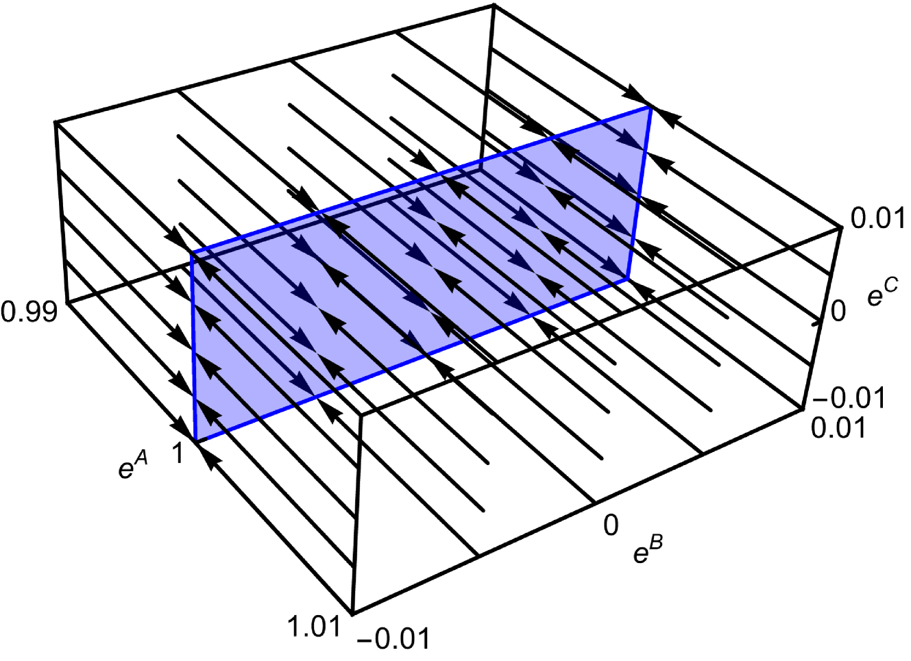
## 3D Vector Field Diagram: Convergence to a Plane
### Overview
The image displays a three-dimensional vector field plot contained within a wireframe box. The plot visualizes a directional flow (represented by black arrows) within a defined volume of space. A prominent, semi-transparent blue plane cuts diagonally through this volume, and the vector field appears to converge toward this plane from both sides.
### Components/Axes
* **Coordinate System:** A 3D Cartesian coordinate system is depicted with three orthogonal axes.
* **Axis Labels & Ranges:**
* **e^A (Vertical Axis):** Labeled on the left side. The scale runs from **0.99** at the bottom to **1.01** at the top. The midpoint tick is labeled **1**.
* **e^B (Horizontal Axis, front):** Labeled along the bottom front edge. The scale runs from **-0.01** on the left to **0.01** on the right. The midpoint tick is labeled **0**.
* **e^C (Depth Axis, right side):** Labeled on the right side. The scale runs from **-0.01** at the bottom to **0.01** at the top. The midpoint tick is labeled **0**.
* **Key Geometric Element:** A **blue, semi-transparent plane** is positioned diagonally within the volume. It is bounded by a blue outline. Its orientation suggests it is defined by a relationship between the e^A, e^B, and e^C variables.
* **Vector Field:** Numerous **black arrows** are distributed throughout the volume. Each arrow has a shaft and an arrowhead indicating direction.
### Detailed Analysis
* **Vector Field Behavior:** The arrows exhibit a uniform, laminar flow pattern. Their primary direction is **toward the blue plane**.
* Arrows located "above" the plane (in the region of higher e^A) point downward and inward toward the plane.
* Arrows located "below" the plane (in the region of lower e^A) point upward and inward toward the plane.
* The flow appears symmetric and convergent from both sides of the plane.
* **Spatial Grounding of the Blue Plane:** The plane is positioned such that it intersects the e^A axis at approximately **e^A = 1**. It is tilted, meaning its intersection with the e^B-e^C plane is a line, not a point. The plane's orientation suggests a linear relationship, likely of the form `e^A = 1 + k1*e^B + k2*e^C` for some constants k1 and k2.
* **Data Point Confirmation:** There are no discrete data points or plotted series. The information is conveyed entirely through the continuous vector field and the reference plane.
### Key Observations
1. **Convergence:** The most salient feature is the convergence of the vector field onto the blue plane. This indicates the plane represents a set of equilibrium points or a stable manifold for the system being visualized.
2. **Narrow Parameter Range:** The axes are zoomed in on a very small region of state space (e^A within ±0.01 of 1, e^B and e^C within ±0.01 of 0). This suggests the analysis is focused on local behavior near the point (e^A=1, e^B=0, e^C=0).
3. **Uniformity:** The vector field appears highly regular and uniform in direction and magnitude (as implied by arrow length) across the displayed volume, suggesting a linear or linearized system.
4. **Diagonal Attractor:** The attractor (the blue plane) is not aligned with any primary axis, indicating the stable dynamics involve a coupled relationship between all three variables (e^A, e^B, e^C).
### Interpretation
This diagram is a technical visualization likely from the fields of dynamical systems, control theory, or stability analysis. It depicts the **local stability** of a system around an equilibrium point located at (e^A=1, e^B=0, e^C=0).
* **What the data suggests:** The vector field shows the instantaneous direction of change for any state within this volume. The consistent flow toward the blue plane demonstrates that if the system is perturbed away from this plane, its dynamics will drive it back toward it. Therefore, the blue plane is a **stable equilibrium manifold**.
* **Relationship between elements:** The axes define the state space variables. The vector field defines the system's governing laws (e.g., differential equations). The blue plane is a geometric representation of the solution set where the system's rate of change is zero (an equilibrium). The convergence of vectors onto it visually proves its stability.
* **Notable implications:** The fact that the attractor is a plane (a 2D surface) within a 3D space, rather than a single point, indicates the system has a **conserved quantity** or a **zero eigenvalue** in its linearization. There is one direction (perpendicular to the plane) in which the system is stable, and two directions (within the plane) where it is neutrally stable or marginally stable. The narrow axis ranges confirm this is a **local analysis**; the global behavior could be different.