## Table: Step-by-Step Constraint and ReLU Adjustment Process
### Overview
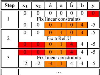
The image displays a technical table illustrating a three-step iterative process for adjusting numerical variables (`x1`, `x2`, `â`, `a`, `b̂`, `b`, `y`) under linear constraints and a ReLU (Rectified Linear Unit) activation function constraint. The table uses color-coding (red and orange) to highlight specific cells undergoing changes or being fixed at each step.
### Components/Axes
* **Structure:** A grid with 8 columns and multiple rows, grouped into three numbered steps (1, 2, 3).
* **Column Headers (Top Row):** `Step`, `x1`, `x2`, `â`, `a`, `b̂`, `b`, `y`.
* **Row Annotations (Between Steps):** Text descriptions of the action taken: "Fix linear constraints" and "Fix a ReLU".
* **Color Key (Implied):**
* **Red Cells:** Likely indicate variables that are being actively modified, are in an error state, or are the focus of the current step's operation.
* **Orange Cells:** Likely indicate variables that are fixed, constrained, or otherwise affected by the operation in that step.
### Detailed Analysis
**Step 1:**
* **Initial State (Top Row of Step 1):** All variables (`x1`, `x2`, `â`, `a`, `b̂`, `b`, `y`) are set to `0`. The cell for `y` is colored **red**.
* **Action:** "Fix linear constraints".
* **Resulting State (Bottom Row of Step 1):** `x1=0`, `x2=0`, `â=0`, `a=1`, `b̂=0`, `b=4`, `y=-5`. The cells for `â`, `a`, `b̂`, `b`, and `y` are colored **orange**.
**Step 2:**
* **Starting State:** Inherits the bottom row from Step 1 (`0, 0, 0, 1, 0, 4, -5`).
* **Action:** "Fix a ReLU".
* **Resulting State (Bottom Row of Step 2):** `x1=0`, `x2=0`, `â=0`, `a=1`, `b̂=4`, `b=4`, `y=-5`. The cells for `x1`, `x2`, `â`, and `b̂` are colored **red**. The cells for `a`, `b`, and `y` are colored **orange**.
**Step 3:**
* **Starting State:** Inherits the bottom row from Step 2 (`0, 0, 0, 1, 4, 4, -5`).
* **Action:** "Fix linear constraints".
* **Resulting State (Bottom Row of Step 3):** `x1=-2`, `x2=-2`, `â=-4`, `a=1`, `b̂=4`, `b=4`, `y=-5`. The cells for `x1`, `x2`, `â`, and `b̂` are colored **red**. The cells for `a`, `b`, and `y` are colored **orange**.
**Final Row (Ellipsis):** The table ends with an ellipsis (`...`), indicating the process may continue beyond the three steps shown.
### Key Observations
1. **Progressive Adjustment:** The process starts from all zeros and iteratively adjusts the variable values. The final output `y` stabilizes at `-5` after Step 1 and remains constant.
2. **Variable Roles:** The variable `a` is set to `1` in Step 1 and never changes. The variable `b` is set to `4` in Step 1 and never changes. This suggests `a` and `b` might be fixed parameters after the initial constraint application.
3. **Focus of Operations:** The "Fix linear constraints" step (Steps 1 & 3) primarily adjusts `x1`, `x2`, `â`, and `b̂`. The "Fix a ReLU" step (Step 2) specifically modifies `b̂` (from `0` to `4`), which then influences the subsequent linear constraint fix in Step 3.
4. **Color Logic:** Red highlights the variables most directly involved in or altered by the current step's core operation. Orange highlights variables that are constrained or hold values resulting from the operation.
### Interpretation
This table demonstrates a **constrained optimization or solving algorithm**, likely for a system involving a linear function (`y = a*x1 + b*x2 + ...` or similar) followed by a ReLU activation (`max(0, value)`). The process alternates between enforcing global linear relationships ("Fix linear constraints") and enforcing the piecewise-linear ReLU condition ("Fix a ReLU").
The data suggests an iterative projection or adjustment method. Starting from an initial guess (all zeros), the algorithm projects the solution onto the set of points satisfying the linear constraints, then projects onto the set satisfying the ReLU constraint, and repeats. The stabilization of `y`, `a`, and `b` indicates convergence for those parameters, while `x1`, `x2`, `â`, and `b̂` continue to be refined. The final values (`x1=-2, x2=-2, â=-4, a=1, b̂=4, b=4, y=-5`) represent a candidate solution that satisfies the sequence of applied constraints shown. The ellipsis implies further iterations might be needed for full convergence or to satisfy additional constraints not depicted.