\n
## Scatter Plot: Average over 8 GLUE tasks for BERT-type models
### Overview
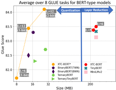
This is a scatter plot comparing the performance (GLUE Score) versus model size (in MB) for various compressed BERT-type models. The chart is divided into two distinct regions by a vertical blue line, illustrating two different compression strategies: "Quantization" (left side) and "Layer Reduction" (right side). Data points represent different model architectures and compression levels, with some points annotated to indicate specific layer counts (L) and bit-widths.
### Components/Axes
* **Title:** "Average over 8 GLUE tasks for BERT-type models"
* **Y-Axis:** Labeled "Glue Score". Scale ranges from 82.0 to 84.0, with major tick marks at 0.5 intervals (82.0, 82.5, 83.0, 83.5, 84.0).
* **X-Axis:** Labeled "Size (MB)". The scale is non-linear, with labeled tick marks at 8, 16, 32, and 200 MB. The region between 32 and 200 MB is compressed.
* **Legend:** Located in the bottom-right quadrant. It lists 8 model types with corresponding color and symbol markers:
* Orange Circle: XTC-BERT*
* Purple Pentagon: BinaryBERT(TWN)
* Dark Purple Diamond: BinaryBERT(BWN)
* Green Hexagon: TernaryBERT
* Light Green Right-Pointing Triangle: TernaryTinyBERT
* Red Circle: XTC-BERT
* Teal X: TinyBERT
* Pink Square: MiniLMv2
* **Annotations & Structural Elements:**
* A thick vertical blue line at approximately 100 MB divides the chart.
* A blue arrow pointing left from the line is labeled "Quantization".
* A blue arrow pointing right from the line is labeled "Layer Reduction".
* Several data points have gray text boxes with arrows pointing to them, indicating model configuration:
* "L=6 (1-bit)" points to the orange circle at ~8 MB.
* "L=12 (1-bit)" points to the orange circle at ~16 MB.
* "L=12 (2-bit)" points to the orange circle at ~32 MB.
* "L=8" points to the red circle at ~200 MB.
* "L=6" points to the red circle at ~200 MB (slightly above the L=8 point).
### Detailed Analysis
**Left Region (Quantization, Size < ~100 MB):**
* **XTC-BERT* (Orange Circles):** Shows a strong positive trend. Performance increases sharply with model size.
* Point 1: Size ≈ 8 MB, Glue Score ≈ 81.8. Annotated as "L=6 (1-bit)".
* Point 2: Size ≈ 16 MB, Glue Score ≈ 83.4. Annotated as "L=12 (1-bit)".
* Point 3: Size ≈ 32 MB, Glue Score ≈ 84.1. Annotated as "L=12 (2-bit)". This is the highest-performing model on the entire chart.
* **BinaryBERT(TWN) (Purple Pentagon):** One point at Size ≈ 16 MB, Glue Score ≈ 82.5.
* **BinaryBERT(BWN) (Dark Purple Diamond):** One point at Size ≈ 16 MB, Glue Score ≈ 83.3.
* **TernaryBERT (Green Hexagon):** One point at Size ≈ 32 MB, Glue Score ≈ 82.7.
* **TernaryTinyBERT (Light Green Triangle):** One point at Size ≈ 16 MB, Glue Score ≈ 82.3.
**Right Region (Layer Reduction, Size ≈ 200 MB):**
* Models in this region are clustered tightly around 200 MB but show a spread in performance.
* **XTC-BERT (Red Circles):** Two points.
* Lower point: Size ≈ 200 MB, Glue Score ≈ 83.3. Annotated as "L=8".
* Higher point: Size ≈ 200 MB, Glue Score ≈ 83.5. Annotated as "L=6".
* **TinyBERT (Teal X):** One point at Size ≈ 200 MB, Glue Score ≈ 83.4.
* **MiniLMv2 (Pink Square):** One point at Size ≈ 200 MB, Glue Score ≈ 83.2.
### Key Observations
1. **Performance-Size Trade-off:** The most dramatic performance gains in the quantization region come from increasing bit-width (1-bit to 2-bit) and layer count (L=6 to L=12) for the XTC-BERT* model, albeit at the cost of increased size.
2. **Efficiency Frontier:** The XTC-BERT* models (orange) form a clear "Pareto frontier" on the left side, offering the best performance for their respective size classes.
3. **Clustering by Strategy:** Models are strictly separated by compression strategy (quantization vs. layer reduction) with no overlap in size.
4. **Performance Range:** The highest score (≈84.1) is achieved by a quantized model (XTC-BERT*, L=12, 2-bit) at 32 MB. The layer-reduced models at 200 MB achieve scores between ≈83.2 and ≈83.5.
5. **Anomaly/Notable Point:** The "L=6" XTC-BERT (red circle) in the layer reduction region performs slightly better than its "L=8" counterpart, which is counterintuitive as fewer layers typically mean a smaller, less capable model. This suggests other factors (like width or training) are at play.
### Interpretation
This chart visually argues for the effectiveness of aggressive quantization (especially the XTC-BERT* approach) as a method for creating highly efficient models. It demonstrates that a 32 MB model using 2-bit quantization can outperform much larger 200 MB models that rely on layer reduction. The data suggests that for the GLUE benchmark, intelligently reducing numerical precision (quantization) may be a more effective compression strategy than simply removing layers, as it achieves superior performance at a fraction of the size. The clear separation of the two strategies highlights a fundamental design choice in model compression: reduce the precision of computations or reduce the number of computational steps. The chart strongly favors the former for this specific task and model family.