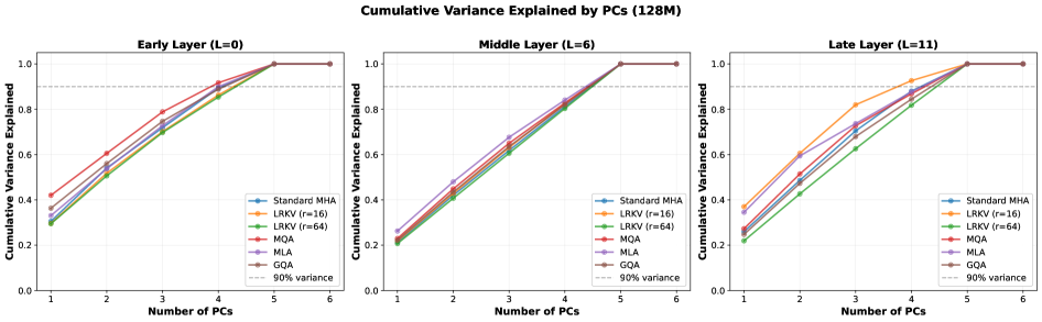
## Line Graphs: Cumulative Variance Explained by PCs (128M) ### Overview The image contains three line graphs comparing the cumulative variance explained by principal components (PCs) across three transformer layers: Early Layer (L=0), Middle Layer (L=6), and Late Layer (L=11). Each graph plots the number of PCs (1–6) against cumulative variance explained (0–1.0), with multiple data series representing different methods. A dashed line at 0.9 (90% variance) serves as a reference threshold. ### Components/Axes - **X-axis**: "Number of PCs" (1–6, integer steps). - **Y-axis**: "Cumulative Variance Explained" (0.0–1.0, linear scale). - **Legend**: Positioned on the right of each subplot, with the following labels and colors: - Standard MHA (blue) - LRKV (r=16) (orange) - LRKV (r=64) (green) - MQA (red) - MLA (purple) - GQA (brown) - 90% variance (gray dashed line). ### Detailed Analysis #### Early Layer (L=0) - **Standard MHA**: Starts at ~0.3 (PC=1), rises steeply to ~1.0 by PC=6. - **LRKV (r=16)**: Begins at ~0.25, surpasses Standard MHA by PC=4 (~0.85). - **LRKV (r=64)**: Starts at ~0.2, reaches ~0.9 by PC=5. - **MQA**: Begins at ~0.35, plateaus at ~0.9 by PC=5. - **MLA**: Starts at ~0.3, reaches ~0.95 by PC=6. - **GQA**: Starts at ~0.3, plateaus at ~0.9 by PC=5. #### Middle Layer (L=6) - **Standard MHA**: Starts at ~0.4, reaches ~1.0 by PC=6. - **LRKV (r=16)**: Begins at ~0.35, surpasses Standard MHA by PC=4 (~0.85). - **LRKV (r=64)**: Starts at ~0.3, reaches ~0.9 by PC=5. - **MQA**: Begins at ~0.4, plateaus at ~0.9 by PC=5. - **MLA**: Starts at ~0.4, reaches ~0.95 by PC=6. - **GQA**: Starts at ~0.4, plateaus at ~0.9 by PC=5. #### Late Layer (L=11) - **Standard MHA**: Starts at ~0.5, reaches ~1.0 by PC=6. - **LRKV (r=16)**: Begins at ~0.45, surpasses Standard MHA by PC=4 (~0.85). - **LRKV (r=64)**: Starts at ~0.4, reaches ~0.9 by PC=5. - **MQA**: Begins at ~0.5, plateaus at ~0.9 by PC=5. - **MLA**: Starts at ~0.5, reaches ~0.95 by PC=6. - **GQA**: Starts at ~0.5, plateaus at ~0.9 by PC=5. ### Key Observations 1. **Consistency Across Layers**: All methods show similar trends, with variance explained increasing as more PCs are added. 2. **Performance Differences**: - **LRKV (r=16)** consistently outperforms other methods in later layers (L=6, L=11), reaching the 90% threshold earlier. - **Standard MHA** performs comparably to other methods in early layers but lags in later layers. - **MQA** and **GQA** plateau earlier than other methods, suggesting diminishing returns. 3. **90% Threshold**: All methods except **LRKV (r=16)** in late layers require 5–6 PCs to exceed 90% variance. ### Interpretation The data suggests that **LRKV (r=16)** is the most efficient method for capturing variance across all layers, particularly in later layers (L=6, L=11), where it achieves higher cumulative variance with fewer PCs. This implies LRKV (r=16) may be better suited for tasks requiring compact representations. In contrast, **Standard MHA** and other methods require more PCs to achieve similar performance, indicating potential inefficiencies in later layers. The consistent plateauing of **MQA** and **GQA** at ~0.9 variance suggests these methods may not scale as effectively for high-dimensional data. The 90% threshold acts as a practical benchmark, highlighting trade-offs between model complexity and performance.