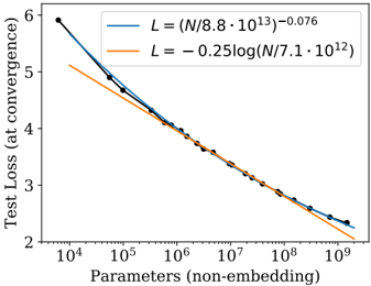
## Line Chart: Scaling Laws for Test Loss vs. Model Parameters
### Overview
The image displays a line chart plotting test loss at convergence against the number of non-embedding parameters for a machine learning model. It compares two theoretical scaling laws (represented by fitted curves) against empirical data points. The chart uses a semi-logarithmic scale (logarithmic x-axis, linear y-axis).
### Components/Axes
* **X-Axis:**
* **Label:** `Parameters (non-embedding)`
* **Scale:** Logarithmic, base 10.
* **Range & Ticks:** Major ticks at `10^4`, `10^5`, `10^6`, `10^7`, `10^8`, `10^9`.
* **Y-Axis:**
* **Label:** `Test Loss (at convergence)`
* **Scale:** Linear.
* **Range & Ticks:** Major ticks at 2, 3, 4, 5, 6.
* **Legend:** Located in the top-right quadrant of the chart area.
* **Blue Line (with circular markers):** Labeled with the equation `L = (N/8.8 * 10^13)^-0.076`. This represents a power-law scaling relationship.
* **Orange Line (solid, no markers):** Labeled with the equation `L = -0.25 log(N/7.1 * 10^12)`. This represents a logarithmic scaling relationship.
* **Data Series:**
* **Empirical Data (Blue Points):** A series of dark blue circular data points connected by a thin blue line. These points represent measured test loss values for models of different sizes.
* **Power-Law Fit (Blue Curve):** A smooth blue curve following the power-law equation, closely tracking the empirical data points.
* **Logarithmic Fit (Orange Curve):** A smooth orange curve following the logarithmic equation.
### Detailed Analysis
**Trend Verification & Data Points:**
1. **Empirical Data / Power-Law Fit (Blue):** This series shows a clear, steeply decreasing trend. The test loss drops rapidly as the number of parameters increases from `10^4` to approximately `10^7`, after which the rate of decrease slows.
* Approximate data points (visually estimated):
* At N ≈ `10^4`: Loss ≈ 5.95
* At N ≈ `10^5`: Loss ≈ 4.9
* At N ≈ `10^6`: Loss ≈ 4.1
* At N ≈ `10^7`: Loss ≈ 3.3
* At N ≈ `10^8`: Loss ≈ 2.7
* At N ≈ `10^9`: Loss ≈ 2.3
2. **Logarithmic Fit (Orange):** This series also shows a decreasing trend, but it is shallower and more linear on this semi-log plot compared to the blue curve. It starts at a lower loss value than the blue curve for small N but decreases at a slower rate.
* The orange line intersects the blue line/data points at approximately N = `10^6` parameters (Loss ≈ 4.1).
* For N < `10^6`, the orange line predicts a lower loss than observed.
* For N > `10^6`, the orange line predicts a higher loss than observed.
### Key Observations
1. **Dominant Trend:** Test loss decreases monotonically with an increase in model parameters (N), following a scaling law.
2. **Model Superiority:** The empirical data (blue points) and its corresponding power-law fit (blue curve) demonstrate a better (lower) test loss than the logarithmic model (orange curve) for all model sizes larger than approximately 1 million (`10^6`) parameters.
3. **Crossover Point:** The two scaling laws predict similar performance around N = `10^6`. Below this size, the logarithmic model is optimistic; above it, the power-law model is more accurate and favorable.
4. **Diminishing Returns:** Both curves show diminishing returns: adding parameters yields smaller reductions in loss as the model grows very large (e.g., the slope flattens between `10^8` and `10^9`).
### Interpretation
This chart provides a quantitative visualization of **neural scaling laws**, a critical concept in modern AI research. It suggests that increasing a model's parameter count is a reliable method for improving performance (reducing test loss), but the relationship is not linear.
* **The Power-Law Fit (Blue):** The equation `L ∝ N^-0.076` indicates a **power-law relationship**. This is a common finding in deep learning, where performance improves as a power of scale (data, compute, or parameters). The exponent (-0.076) quantifies the rate of improvement.
* **The Logarithmic Fit (Orange):** The equation `L ∝ -log(N)` suggests a **logarithmic relationship**, which would imply even more severe diminishing returns than a power law. The chart clearly shows this model is a poorer fit for the empirical data beyond the crossover point.
* **Practical Implication:** The data strongly supports investing in scaling models beyond the `10^6` parameter range, as the power-law trend continues to yield meaningful performance gains up to at least `10^9` parameters, outperforming the more pessimistic logarithmic projection. The chart serves as evidence for the efficacy of large-scale model training.