## Line Graphs: Model Performance Across Parameter Values
### Overview
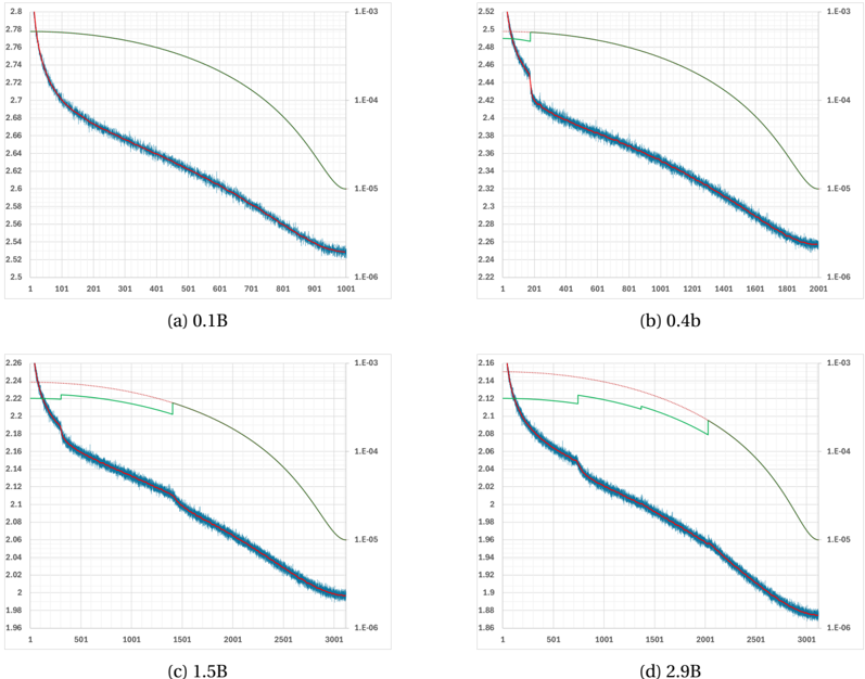
The image contains four line graphs labeled (a) 0.1B, (b) 0.4B, (c) 1.5B, and (d) 2.9B. Each graph plots "Value" (logarithmic scale: 1e-6 to 2.8) against "Time" (linear scale: 1 to 3001). Three data series are represented: Model A (blue), Model B (green), and Model C (red). All graphs share identical axis labels and legend placement (top-right), but vary in time range and value trends.
---
### Components/Axes
- **Y-Axis**: "Value" (logarithmic scale: 1e-6, 1e-5, 1e-4, ..., 2.8)
- **X-Axis**: "Time" (linear scale: 1, 101, 201, ..., 3001)
- **Legend**: Top-right corner, labels:
- Model A: Blue line
- Model B: Green line
- Model C: Red line
---
### Detailed Analysis
#### Graph (a) 0.1B
- **Model A (Blue)**: Starts at ~2.8, decreases linearly to ~2.5 over 1001 time units.
- **Model B (Green)**: Sharp drop from ~2.8 to ~2.5 by time 101, then plateaus.
- **Model C (Red)**: Gradual decline from ~2.8 to ~2.5 over 1001 time units.
#### Graph (b) 0.4B
- **Model A (Blue)**: Starts at ~2.5, decreases linearly to ~2.2 over 2001 time units.
- **Model B (Green)**: Sharp drop from ~2.5 to ~2.2 by time 201, then plateaus.
- **Model C (Red)**: Gradual decline from ~2.5 to ~2.2 over 2001 time units.
#### Graph (c) 1.5B
- **Model A (Blue)**: Starts at ~2.2, decreases linearly to ~1.9 over 3001 time units.
- **Model B (Green)**: Sharp drop from ~2.2 to ~1.9 by time 301, then plateaus.
- **Model C (Red)**: Gradual decline from ~2.2 to ~1.9 over 3001 time units.
#### Graph (d) 2.9B
- **Model A (Blue)**: Starts at ~1.9, decreases linearly to ~1.6 over 3001 time units.
- **Model B (Green)**: Sharp drop from ~1.9 to ~1.6 by time 301, then plateaus.
- **Model C (Red)**: Gradual decline from ~1.9 to ~1.6 over 3001 time units.
---
### Key Observations
1. **Model B (Green)** exhibits a consistent pattern: rapid initial decline followed by stabilization, regardless of parameter value.
2. **Model A (Blue)** and **Model C (Red)** show linear decay, with slower rates as parameter values increase.
3. **Parameter Correlation**: Higher parameter values (e.g., 2.9B) correlate with longer timeframes to reach plateau/stable values.
4. **Logarithmic Scale**: Y-axis compression emphasizes early-time dynamics, making late-time changes appear less pronounced.
---
### Interpretation
- **Model Behavior**: Model B’s sharp drop suggests a threshold effect or rapid adaptation, while Models A and C reflect steady-state decay.
- **Parameter Impact**: Larger parameters (e.g., 2.9B) delay stabilization, implying slower system response or increased complexity.
- **Anomalies**: No outliers detected; all models follow predictable trends. The green line’s plateau in all graphs indicates a potential equilibrium state.
- **Practical Implications**: The parameter value likely governs system sensitivity or resource allocation, with Model B optimizing for rapid initial adjustment.