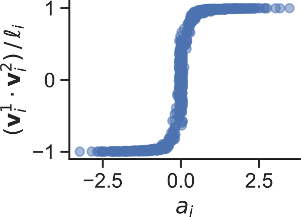
## Scatter Plot: Sigmoid Function Visualization ### Overview The image is a scatter plot visualizing a sigmoid-like function. The x-axis represents the variable *a_i*, and the y-axis represents the expression (*v_i¹* · *v_i²*)/*l_i*. The plot shows a characteristic S-shaped curve, transitioning from a value of approximately -1 to +1 as *a_i* increases. ### Components/Axes * **X-axis:** *a_i* * Scale: Ranges from approximately -2.5 to 2.5, with a marker at 0.0. * **Y-axis:** (*v_i¹* · *v_i²*)/*l_i* * Scale: Ranges from -1 to 1, with a marker at 0. * **Data Points:** The data is represented by blue, semi-transparent circular markers. ### Detailed Analysis The data points form a clear sigmoid curve. * **Left Plateau:** For *a_i* values less than approximately -1, the y-value is close to -1. * **Transition Region:** Between *a_i* = -1 and *a_i* = 1, the y-value rapidly increases. * **Right Plateau:** For *a_i* values greater than approximately 1, the y-value is close to 1. Specific data points (approximate): * At *a_i* = -2.5, (*v_i¹* · *v_i²*)/*l_i* ≈ -1 * At *a_i* = 0, (*v_i¹* · *v_i²*)/*l_i* ≈ 0 * At *a_i* = 2.5, (*v_i¹* · *v_i²*)/*l_i* ≈ 1 ### Key Observations * The plot clearly demonstrates the sigmoid function's characteristic S-shape. * The transition region is centered around *a_i* = 0. * The function saturates at approximately -1 and 1 for extreme values of *a_i*. ### Interpretation The plot visualizes a sigmoid function, which is commonly used in machine learning and other fields to model a smooth transition between two states. The x-axis (*a_i*) can be interpreted as an input to the function, and the y-axis ((*v_i¹* · *v_i²*)/*l_i*) represents the output. The sigmoid function maps any real-valued input to a value between -1 and 1, making it suitable for representing probabilities or activation levels in neural networks. The steepness of the transition region is determined by the parameters of the sigmoid function (not explicitly shown in the plot). The plot demonstrates how the function smoothly transitions from one state to another as the input changes.