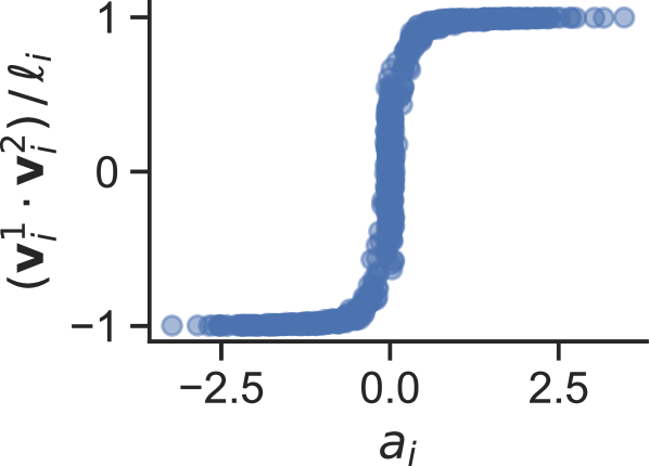
\n ## Scatter Plot: Relationship between a_j and (v_i^-1 ⋅ v_i^-1) / l_i ### Overview The image presents a scatter plot illustrating the relationship between two variables: a_j on the x-axis and (v_i^-1 ⋅ v_i^-1) / l_i on the y-axis. The plot shows a distinct sigmoidal or "S" shaped curve, indicating a non-linear relationship between the two variables. The data points are clustered, forming a clear pattern. ### Components/Axes * **X-axis Label:** a_j * Scale: Approximately ranges from -2.75 to 2.75. * Markers: -2.5, 0.0, 2.5 * **Y-axis Label:** (v_i^-1 ⋅ v_i^-1) / l_i * Scale: Approximately ranges from -1.2 to 1.2. * Markers: -1, 0, 1 * **Data Points:** Blue circles, representing individual data observations. * **Background:** White. ### Detailed Analysis The data exhibits a clear transition between two distinct states. * **Left Side (a_j < 0):** For values of a_j less than approximately 0, the value of (v_i^-1 ⋅ v_i^-1) / l_i remains relatively constant at approximately -1. There is some scatter, but the points cluster tightly around this value. * **Transition Region (a_j ≈ 0):** As a_j approaches 0, there is a rapid increase in (v_i^-1 ⋅ v_i^-1) / l_i. This region is characterized by a high density of data points and a steep slope. The transition appears to occur over a range of approximately -0.5 to 0.5 for a_j. * **Right Side (a_j > 0):** For values of a_j greater than approximately 0, the value of (v_i^-1 ⋅ v_i^-1) / l_i plateaus at approximately 1. Similar to the left side, the points are clustered around this value, with some scatter. There are no explicit data points listed, but the trend is clear. ### Key Observations * The plot demonstrates a threshold effect. The value of (v_i^-1 ⋅ v_i^-1) / l_i remains near -1 until a_j reaches a certain threshold (around 0), at which point it rapidly increases to approximately 1. * The transition is not instantaneous but occurs over a small range of a_j values. * The data is relatively clean, with no obvious outliers. ### Interpretation This plot likely represents a system exhibiting a switching behavior. The variable a_j could be an input parameter or control variable, and (v_i^-1 ⋅ v_i^-1) / l_i could be an output or response variable. The sigmoidal shape suggests that the system transitions between two states based on the value of a_j. The variables themselves are not immediately interpretable without further context. However, the form of the equation (v_i^-1 ⋅ v_i^-1) / l_i suggests that v_i represents a velocity or rate, and l_i represents a length or distance. The inverse squared velocity divided by length could represent a form of energy or power. The plot could be modeling a physical system, a biological process, or a computational model. The threshold behavior suggests a form of activation or triggering mechanism. The steepness of the transition indicates a sensitive response to changes in a_j near the threshold.