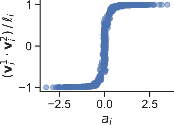
## Scatter Plot: (v_i^1 · v_i^2)/λ_i vs a_j ### Overview The image depicts a scatter plot with a step-like curve. Data points are clustered near y = -1 for a_j < -0.5, transition sharply to y = 1 for a_j > 0.5, with a gradual transition between a_j = -0.5 and 0.5. The plot uses blue circular markers and includes a legend for the data series. ### Components/Axes - **X-axis (a_j)**: Labeled "a_j" with ticks at -2.5, -1.5, -0.5, 0.0, 0.5, 1.5, 2.5. Scale ranges from -2.5 to 2.5. - **Y-axis ((v_i^1 · v_i^2)/λ_i)**: Labeled "(v_i^1 · v_i^2)/λ_i" with ticks at -1, 0, 1. Scale ranges from -1 to 1. - **Legend**: Located in the top-right corner, showing a blue line with circular markers labeled "Data Series". ### Detailed Analysis - **Data Points**: - For a_j < -0.5: All points cluster at y = -1 (e.g., a_j = -2.5, y = -1; a_j = -1.5, y = -1). - Transition Region (-0.5 ≤ a_j ≤ 0.5): Points gradually shift from y = -1 to y = 1. Example: a_j = -0.3, y ≈ -0.8; a_j = 0.3, y ≈ 0.8. - For a_j > 0.5: All points cluster at y = 1 (e.g., a_j = 1.5, y = 1; a_j = 2.5, y = 1). - **Uncertainty**: The transition region spans approximately a_j = -0.5 to 0.5, with no clear boundary. The sharpest change occurs near a_j = 0. ### Key Observations 1. **Step Function Behavior**: The plot exhibits a binary-like response, with y ≈ -1 for negative a_j and y ≈ 1 for positive a_j. 2. **Transition Sharpness**: The transition occurs over a narrow interval (Δa_j ≈ 1), suggesting a threshold effect. 3. **Data Density**: Points are densely packed in the transition region, indicating variability or measurement uncertainty. ### Interpretation The plot likely represents a threshold-dependent relationship between a_j and the normalized dot product (v_i^1 · v_i^2)/λ_i. The sharp transition at a_j ≈ 0 suggests a critical point or phase boundary in the system being modeled. The uncertainty in the transition region (a_j = -0.5 to 0.5) could reflect: - Measurement noise in experimental data - Model parameter sensitivity - A probabilistic boundary (e.g., 50% probability of y = 1 at a_j = 0) The mathematical expressions imply a geometric or algebraic relationship, possibly involving vectors (v_i^1, v_i^2) and a scaling factor λ_i. This could relate to: - Normalized similarity metrics in machine learning - Phase transitions in physics (e.g., Ising model) - Binary classification boundaries in signal processing The absence of a smooth gradient outside the transition region suggests the system exhibits bistable or binary behavior, with a_j acting as a control parameter modulating the state.