## Image Analysis: Positive and Negative Class Examples ### Overview The image presents two examples of handwritten digits, one labeled as a "positive class" and the other as a "negative class." The positive class example (a digit '1') has colored horizontal lines overlaid on it. The negative class example (a digit '0') is shown without any overlays. The image also includes the notation "p = 1, r = 1" below the examples. ### Components/Axes * **Positive Class:** A handwritten digit '1' with colored horizontal lines overlaid. * **Negative Class:** A handwritten digit '0'. * **Labels:** "positive class", "negative class", "p = 1, r = 1" * **Colored Lines (Positive Class):** The digit '1' has several short, horizontal lines of different colors overlaid on it. The colors appear to be: * Red * Blue * Green * Teal * Purple * Yellow ### Detailed Analysis or ### Content Details * **Positive Class (Digit '1'):** The digit '1' is slightly slanted. The colored lines are positioned horizontally across the digit. * **Negative Class (Digit '0'):** The digit '0' is a closed loop. * **Text:** The text "positive class" is located below the digit '1'. The text "negative class" is located below the digit '0'. The text "p = 1, r = 1" is located below both examples, centered. ### Key Observations * The positive class example has colored lines overlaid, while the negative class example does not. * The notation "p = 1, r = 1" likely refers to parameters or values associated with the classification or data generation process. ### Interpretation The image illustrates the concept of positive and negative classes in a classification problem, likely related to digit recognition. The colored lines on the positive class example might represent features or attributes that are important for identifying the digit '1'. The "p = 1, r = 1" notation suggests specific parameter settings used in this example. The image highlights the distinction between a positive instance (digit '1') and a negative instance (digit '0') within the context of a machine learning or pattern recognition task.

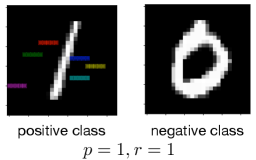
## Diagram: Binary Classification Representation ### Overview The image is a conceptual diagram illustrating two distinct classes in a binary classification problem. It visually contrasts the spatial distribution of data points belonging to a "positive class" versus a "negative class." The diagram includes a performance metric at the bottom. ### Components/Axes The image is divided into two primary panels side-by-side on a black background, with a line of text centered below them. 1. **Left Panel (Positive Class):** * **Visual Element:** A thick, white diagonal line runs from the bottom-left to the top-right. Intersecting this line are several short, horizontal colored bars. * **Colors Observed (from top to bottom):** Red, Green, Blue, Purple. * **Label:** The text "positive class" is centered directly below this panel. 2. **Right Panel (Negative Class):** * **Visual Element:** A thick, white, irregular ring or oval shape with a black center. The shape is not a perfect circle and has a slightly jagged or pixelated edge. * **Label:** The text "negative class" is centered directly below this panel. 3. **Bottom Text:** * **Content:** The mathematical notation `p = 1, r = 1` is centered at the very bottom of the entire image, beneath both class labels. ### Detailed Analysis * **Positive Class Representation:** The data points (represented by colored bars) are arranged linearly along a clear diagonal decision boundary (the white line). This suggests a feature space where the positive class is linearly separable. The different colors (red, green, blue, purple) may represent different sub-categories, features, or instances within the positive class, but no legend is provided to define them. * **Negative Class Representation:** The data forms a continuous, ring-like cluster. This represents a non-linear distribution where the negative class occupies a region surrounding a central void. This is a classic example of data that is not linearly separable from a central point. * **Performance Metric:** The text `p = 1, r = 1` is standard notation for **Precision (p)** and **Recall (r)**. A value of 1 for both indicates perfect classification performance on a given dataset: no false positives (Precision = 1) and no false negatives (Recall = 1). ### Key Observations 1. **Contrasting Geometries:** The core visual message is the stark contrast between a linearly organized class (positive) and a non-linear, clustered class (negative). 2. **Perfect Scores:** The stated precision and recall of 1.0 imply that, for the data this diagram represents, a classifier has achieved flawless separation between these two geometrically distinct classes. 3. **Color Usage:** Colors are used only in the positive class panel, potentially to highlight individual data points or subgroups. The negative class is monochromatic (white). 4. **Spatial Layout:** The legend/labels are placed directly below their respective visual components. The performance metric is placed centrally at the bottom, acting as a summary for the entire classification result. ### Interpretation This diagram is a pedagogical or conceptual illustration, not a plot of empirical data. Its purpose is to visually communicate the idea of class separability in machine learning. * **What it demonstrates:** It shows that perfect classification (`p=1, r=1`) is achievable when two classes have fundamentally different and non-overlapping geometric structures in the feature space—one is a line, the other is a ring. * **Relationship between elements:** The left and right panels are direct counterparts, showing the two possible outcomes of a binary classifier. The bottom text (`p=1, r=1`) is the quantitative result of successfully distinguishing between the two visual patterns shown above. * **Underlying Message:** The image likely serves to explain a concept like the "kernel trick" in Support Vector Machines (SVMs) or the need for non-linear models. It visually argues that while a simple linear boundary (the white line) can define the positive class, a more complex, non-linear boundary is required to encapsulate the negative class (the ring). The perfect scores suggest that with the right model or feature transformation, such distinct patterns can be perfectly classified.

## Diagram: Binary Classification Visualization ### Overview The image depicts a binary classification scenario with two distinct regions labeled "positive class" and "negative class." Each region contains a pixelated shape and associated visual elements. Below both regions, the text "p = 1, r = 1" is displayed, likely indicating precision (p) and recall (r) metrics. ### Components/Axes - **Left Region (Positive Class)**: - Label: "positive class" (centered below the region). - Visual Elements: - A vertical white line (diagonal orientation) occupying the central portion. - Five colored horizontal rectangles (red, green, blue, yellow, purple) aligned to the left of the line. - **Right Region (Negative Class)**: - Label: "negative class" (centered below the region). - Visual Elements: - A pixelated circular shape (white with black background). - **Text Below**: - "p = 1, r = 1" (centered below both regions). ### Detailed Analysis - **Positive Class**: - The vertical line and colored rectangles suggest a structured or segmented representation, possibly indicating features or attributes. - No explicit legend or axis markers are present, but the colored rectangles may imply categorical data (e.g., feature importance or thresholds). - **Negative Class**: - The circular shape is uniform and lacks additional annotations, suggesting a simpler or more homogeneous representation. - **Text**: - "p = 1, r = 1" implies perfect precision and recall, though this is unusual in real-world scenarios and may represent an idealized or synthetic example. ### Key Observations 1. The positive class is visually more complex (line + colored bars) compared to the negative class (single shape). 2. The absence of a legend or axis scales limits quantitative interpretation of the colored rectangles. 3. The text "p = 1, r = 1" is the only explicit numerical data, but its validity depends on context not provided in the image. ### Interpretation This diagram likely illustrates a simplified binary classification task, where the positive class is represented by a structured pattern (line and colored bars) and the negative class by a circular shape. The "p = 1, r = 1" values suggest an idealized model with no false positives or negatives, which is unrealistic in practice. The colored rectangles in the positive class may symbolize distinct features or decision boundaries, but their exact meaning is unclear without additional context. The image emphasizes visual differentiation between classes rather than quantitative analysis.